IDEAS Tutorial
This tutorial is an instructional guide designed for self-guided onboarding to the IDEAS platform. The guide is a step-by-step walkthrough for new users to set up, manage, and analyze data in IDEAS.
By following this guide, you will learn how to:
- Set up and organize new projects and data tables for your data analysis.
- Upload, manage, and use IDEAS intuitive design to correctly assign various file types, including miniscope movies, behavioral recordings, and annotation files.
- Prepare your data for analysis by processing your recordings, identifying cells using the CNMF-E workflow and ensuring data quality with the Calcium Imaging QC Report tool.
- Synchronize neural and behavioral data, and use analysis tools such as Map Annotations To ISXD Data, Zone Occupancy Analysis, Peri-Event Analysis and Compare Neural Activity Across States.
Tips as you walk through this document:
- Click on links for additional documentation.
- This guide will use highlighted numbers (e.g., [1], [2], etc.) to reference the IDEAS Flowchart.
- For the purpose of this tutorial, download the miniscope movie and behavioral files from this link.
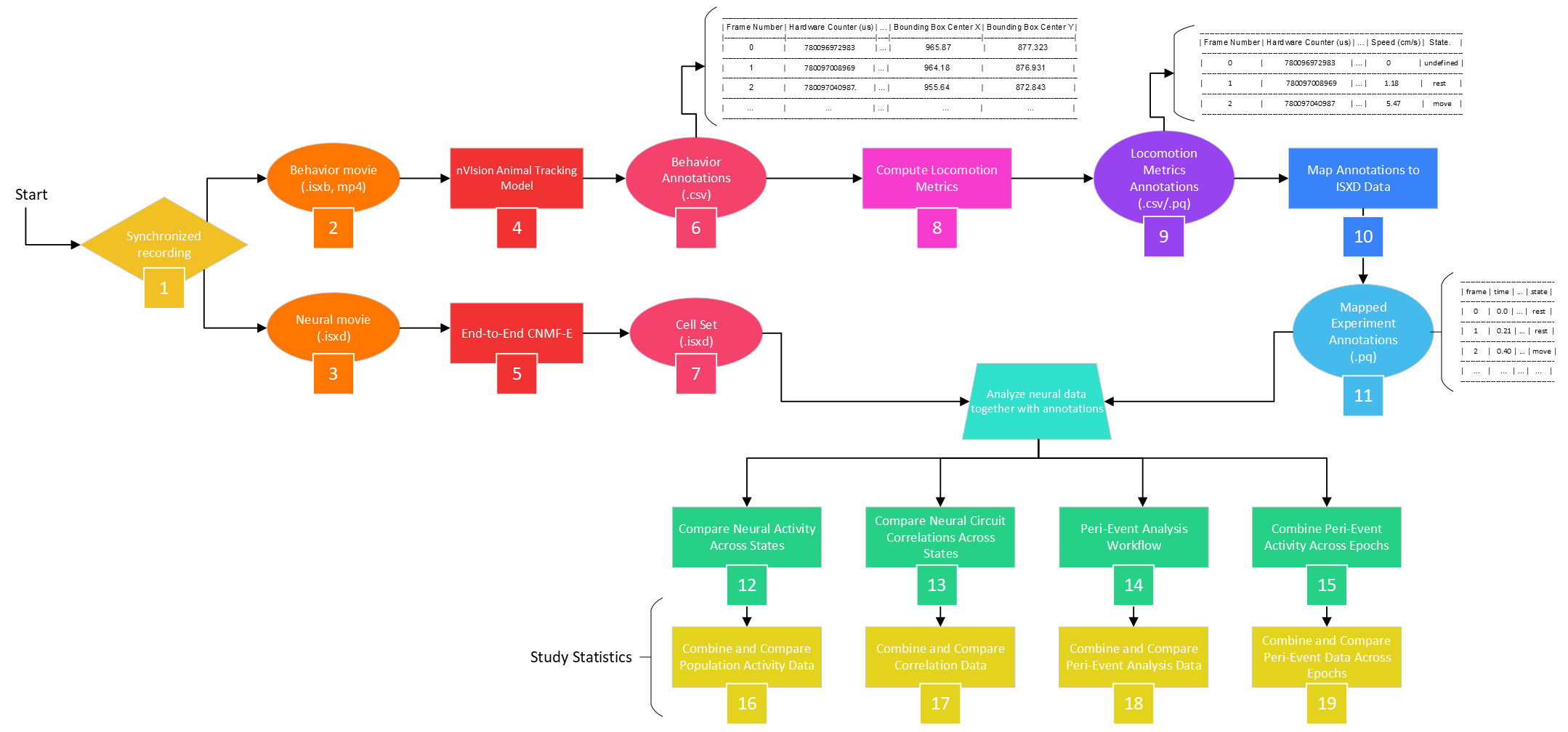
Flowchart
Reference the following flowchart when using this tutorial. The numbers in brackets correspond to the respective numbers in the chart.
Start a Project
Goal
Begin by creating a new project in IDEAS. This section shows you how to set up your workspace and create your first data table for organizing your recordings.
1. Create a new project by selecting  at the top right corner of the IDEAS Projects page. Often, a project corresponds to all the data and analyses for a scientific publication. Enter the project name ("Demo from scratch: Small Cohort") and click
  .
.
2. Once you create a new project, you'll be prompted to 'Create your first data table.' Enter the name ("Small Cohort") for this table, then click .
Upload Files
Goal
Learn how to upload your neural and behavioral data files in this section. You’ll see how to assign file types and make sure everything is ready for analysis.
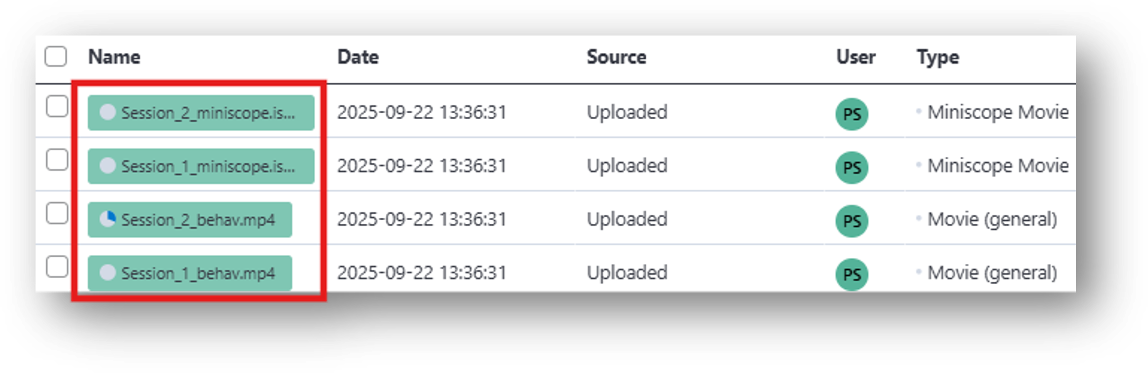
3. From the newly generated data table, go to  at the bottom left, then either drag or select your miniscope and behavioral files to upload into the File Browser. These correspond to the [2] Behavior Movie (.isxb, .mp4) and [3] Neural Movie (.isxd) in the IDEAS flowchart. You can monitor the status of the upload in the File Browser as the grey circle next to the filename turns blue.
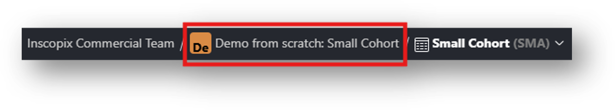
Files can also be accessed from the main project page of Demo from scratch: Small Cohort. To do so:
- Select the project name from the folder tree along the top of the browser.
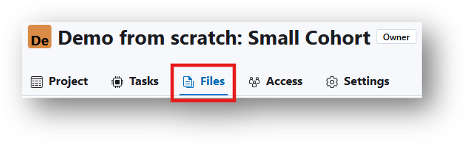
- Select Files from the top menu:
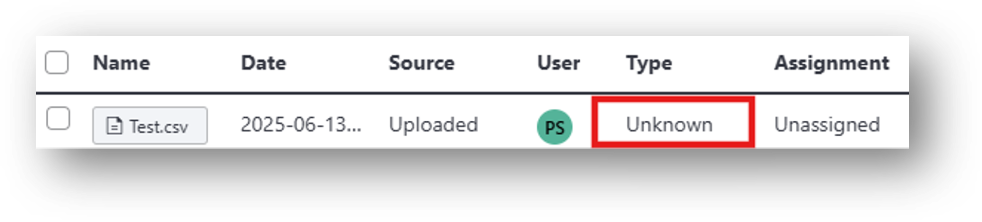
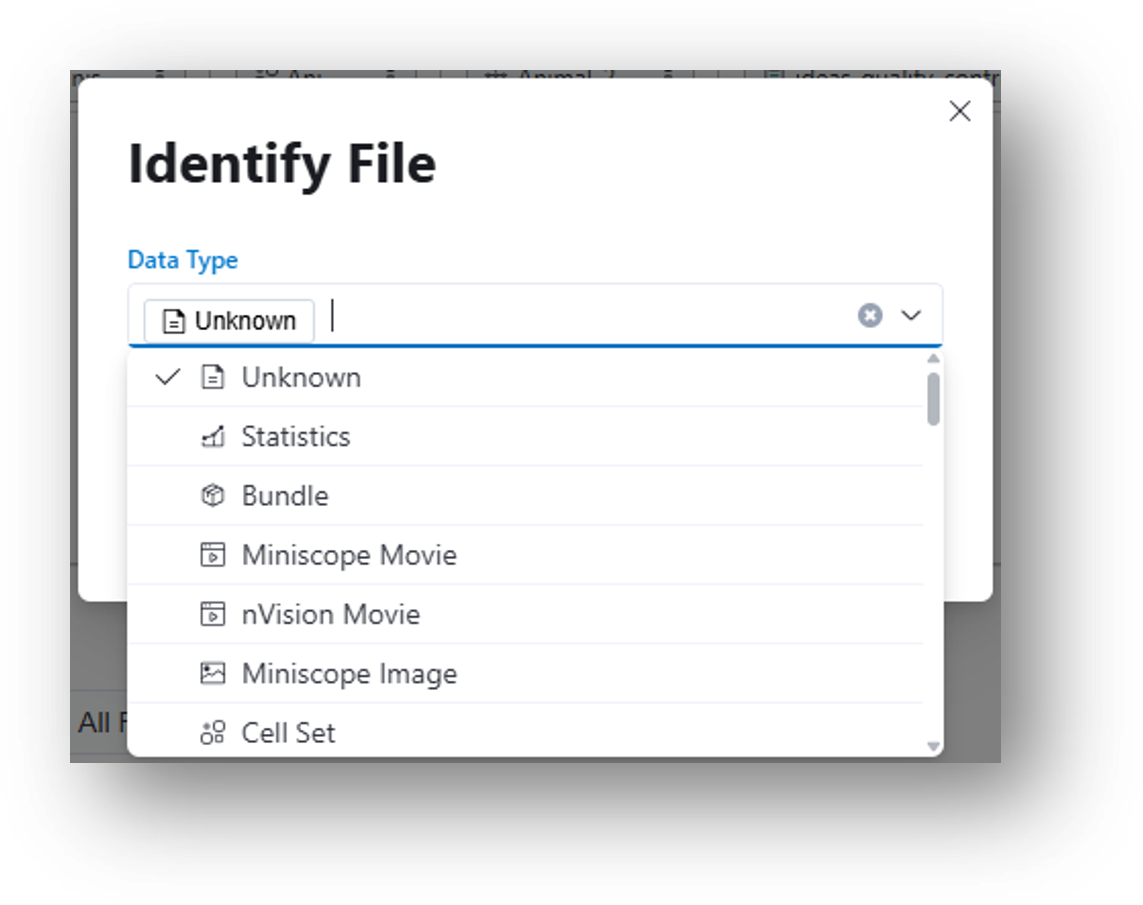
IDEAS accepts any file format (e.g., .isxd, .gpio, .imu, .csv, .mp4). For example, you can upload videos from your external behavior camera as well as manual scoring or annotation files generated outside of IDEAS. These scoring/annotation files would correspond to [6] Behavior Annotations in the IDEAS flowchart. Note: IDEAS may not automatically identify the file type or generate previews for certain uploads. For instance, a file with a .csv extension could be one of several file types and is therefore labeled 'Unknown' by default.
You will need to manually specify the file type by clicking the ![]() Change file type icon in the File Browser and selecting a file type from the menu as illustrated below. Selecting a supported file type will trigger preview generation and metadata extraction, if applicable.
Change file type icon in the File Browser and selecting a file type from the menu as illustrated below. Selecting a supported file type will trigger preview generation and metadata extraction, if applicable.
Organize Data
Goal
This section explains how to structure your data tables, add rows and columns, and link your files to each recording session for easy access and analysis.
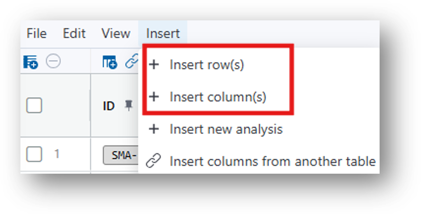
4. A row in a data table contains a collection of related data. This is often, but not limited to, neural and behavioral recordings, animal ID numbers, assorted experimental details, etc. In the Small Cohort data table, each row will correspond to all realted data from a single recording session. Create columns for your movie and behavioral files, as well as enough rows for two recordings:
- Insert>Insert column(s)>Column Type 'File'>Data Type 'Miniscope Movie'>Insert
- Insert>Insert column(s)>Column Type 'File'>Data Type 'Movie (general)'>Insert If you used an nVision to record your behavior movie, you can select the Data Type 'nVision Movie.'
- Insert>Insert row(s)>Number of rows=1
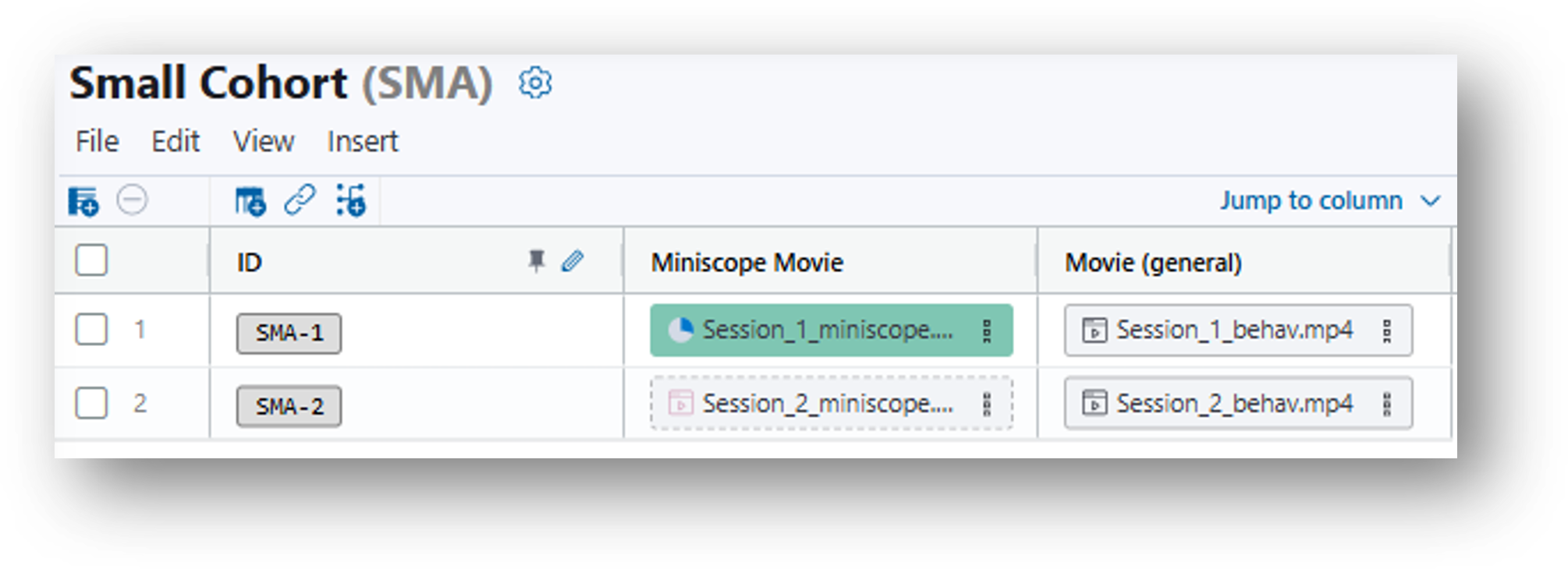
The resulting table looks as follows:
![]()
5. Populate the rows. Drag and drop the miniscope movies and the corresponding behavior movies from the File Browser to the same row of your data table.
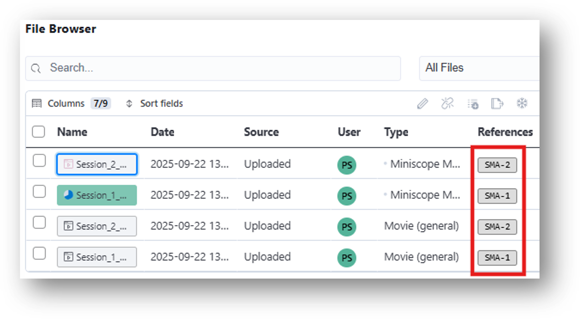
6. Note that when the files are dropped in the data table, the Assignment column in the File Browser changes from 'Unassigned' to 'SMA-1' or 'SMA-2.'
Analyze Neural Activity Data
Goal
In this section you will learn how to prepare and analyze your neural recordings through a process that ensures data quality and enables reliable downstream analysis.
7. Create an analysis table to identify cells from the miniscope movies in your data table. In this example, we'll use CNMF-E to perform cell extraction. This step corresponds to [5] Cell Identification Workflow in the IDEAS flowchart.
- Navigate to your original data table. Then select Insert>Insert new analysis or click the
 Insert New Analysis icon and a popup window will appear entitled 'Create Analysis Table.'
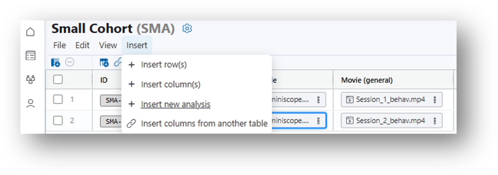
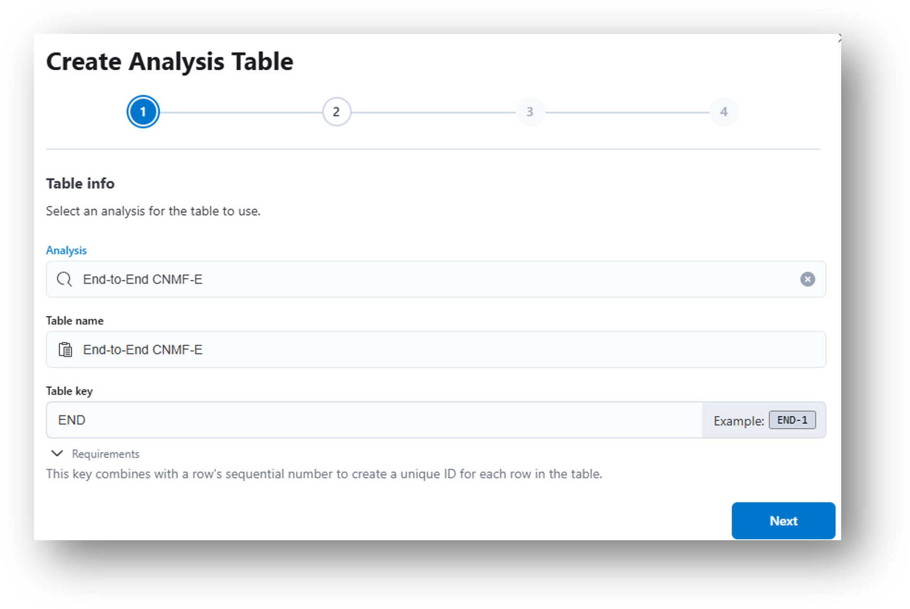
- (Step 1) Under the Analysis dropdown menu, select End-to-End CNMF-E. Click Next.
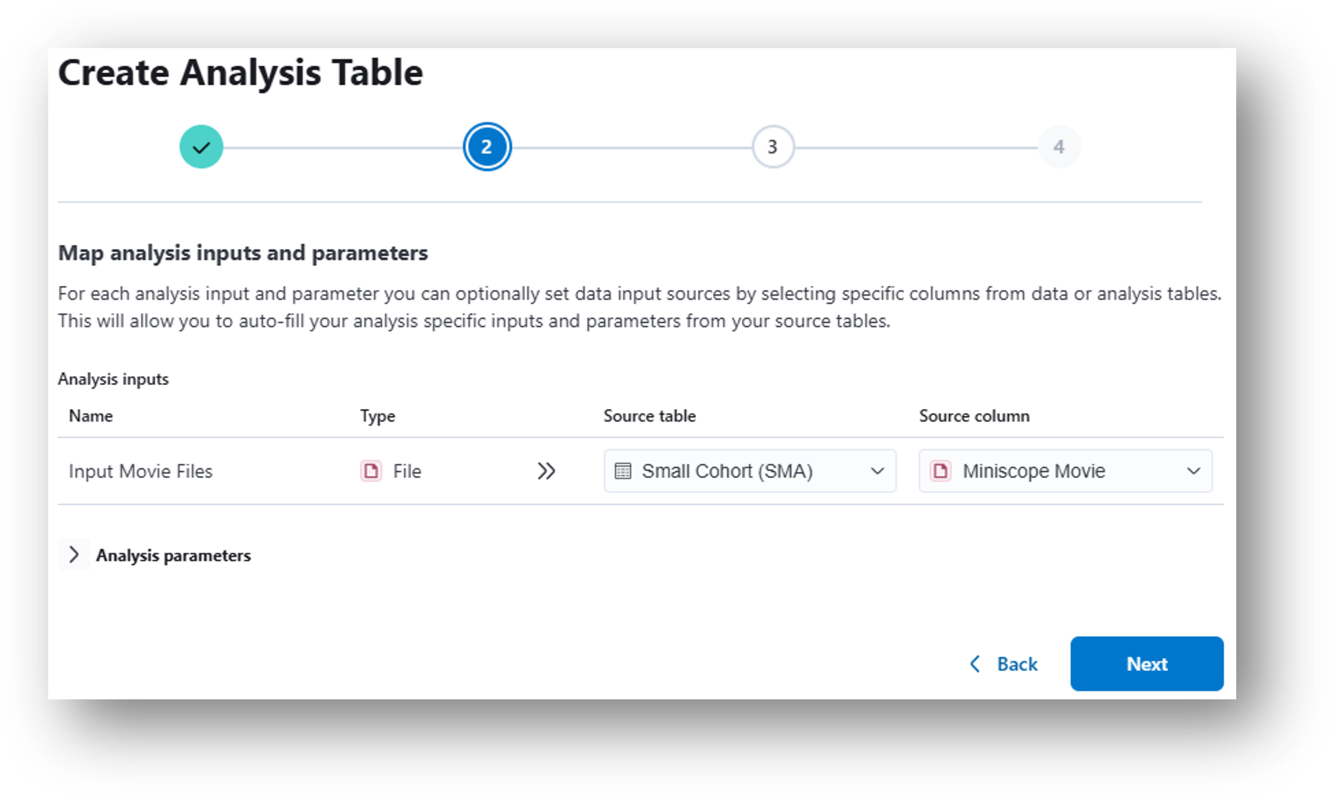
- (Step 2) In the following popup window, select Miniscope Movie from the Source column dropdown menu. Click Next.
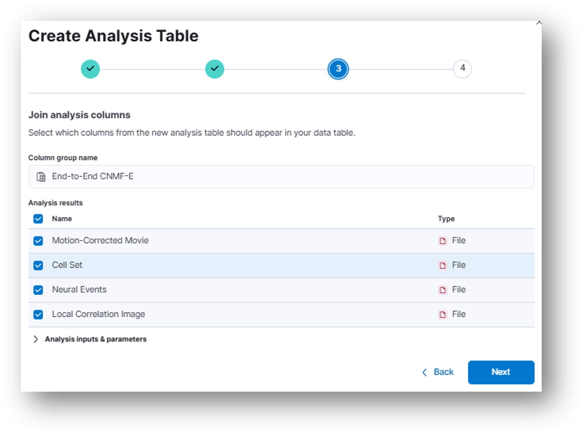
- (Step 3) In the next popup window, you can select which columns you would like to include from the new analysis table in your currently selected data table.
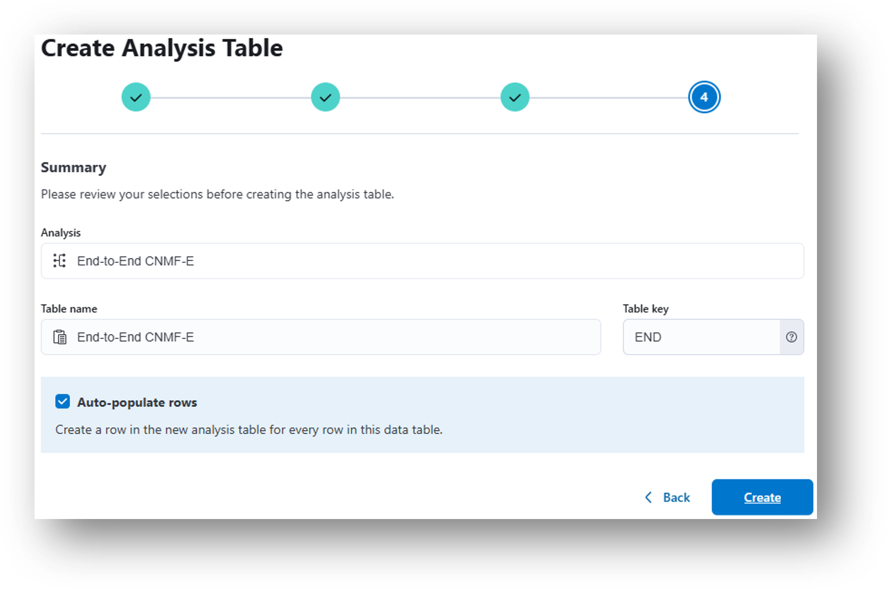
- (Step 4) Review the details and click Create to generate the analysis table.
Note
Alternatively, you can create an analysis table (or another data table) from scratch by navigating to the main project page and selecting + Add, then either Data table or Analysis table.
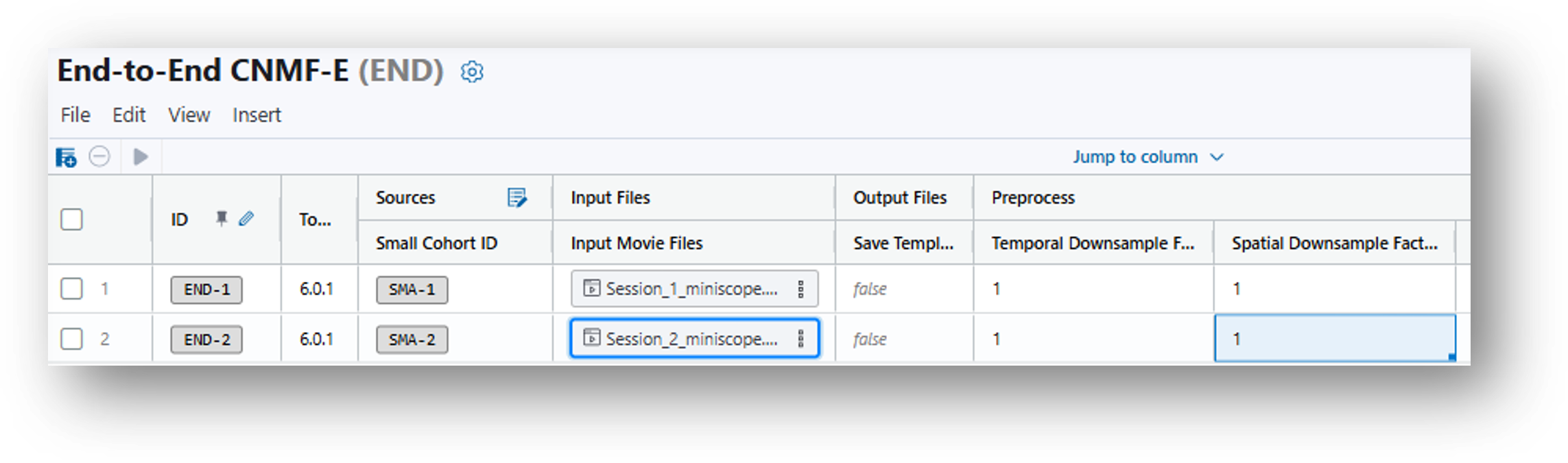
8. Having created the End-to-End CNMF-E analysis table, there will be a row for every recording in the original data table. The parameters, listed in columns to the right of the Input Files, will be populated by default suggestions and can be adjusted according to your needs. Please refer to the End-to-End CNMFe documentation and/or this iQ page for info on each parameter. In the case of the demo files, it is recommended that you set the Temporal Downsample Factor and Spatial Downsample Factor to 1, as the files have already been sized for faster file transfer speed.
9. Having done so, click the  button on the bottom right-hand corner of the window to run the analysis.
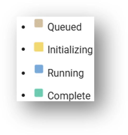
The task is complete when the color square to the right of the window progresses from tan (Queued) to green (Complete).
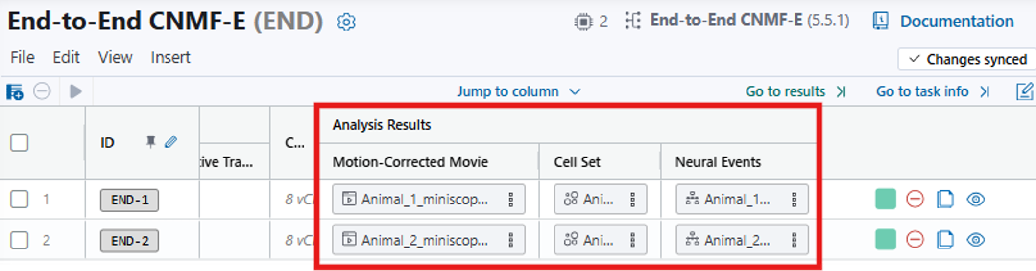
When the analysis is complete, the results will populate the corresponding columns of the analysis table. The results in the Cell Set column correspond to [7] Cell Set (.isxd) in the IDEAS flowchart.
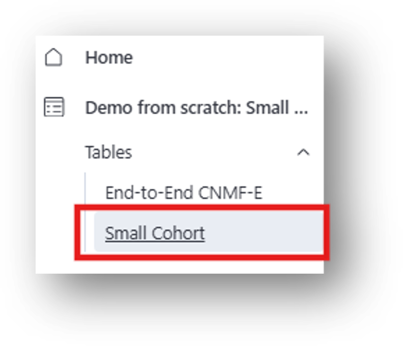
10. Please note that the results are also appended to the Small Cohort Data Table. To navigate directly to the Small Cohort Data Table, expand the left-hand menu by selecting  on the top left corner of the browser, then select Small Cohort from the project dropdown.
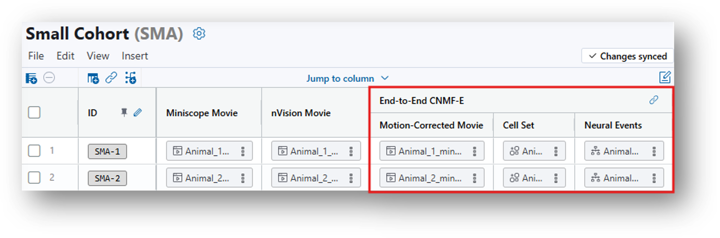
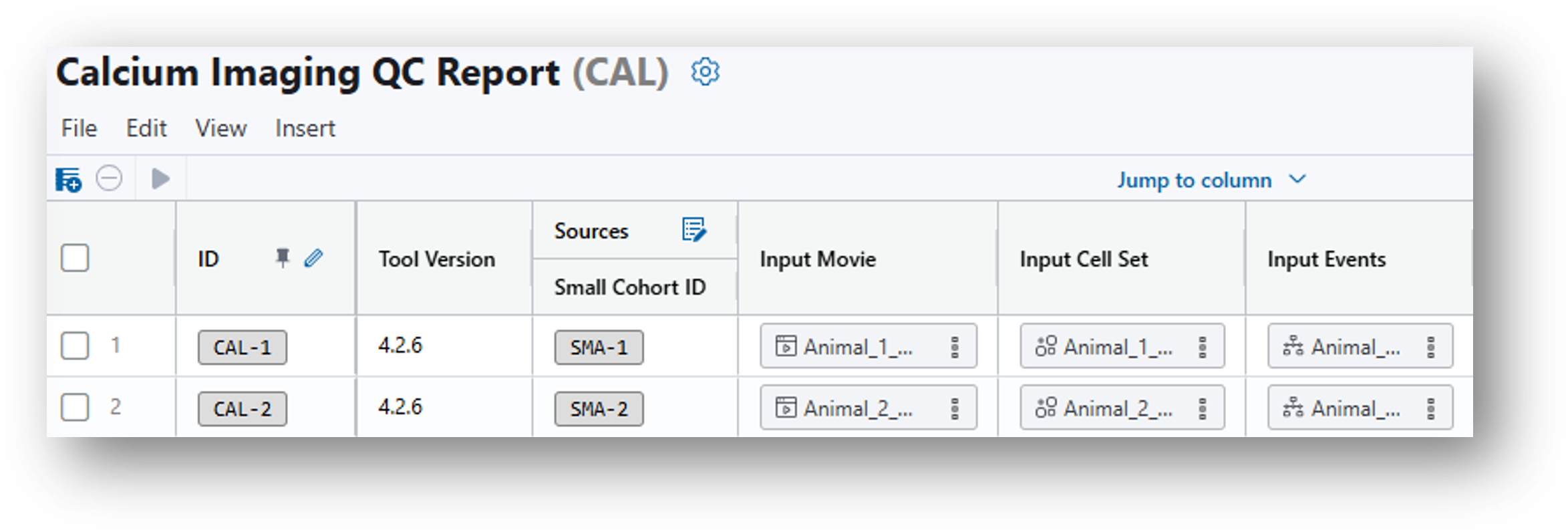
11. Scroll to the right and you can access the End-to-End CNMF-E results:
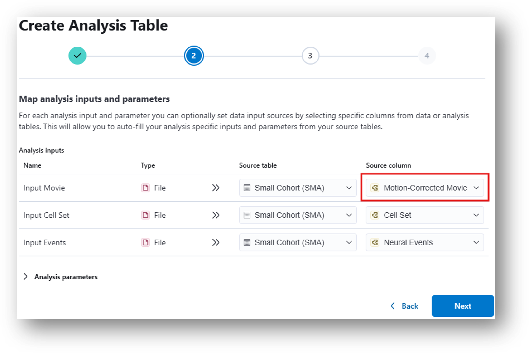
12. Having navigated back to the Small Cohort Data Table, create and run a Calcium Imaging QC Report analysis table following the same steps as you went through to create the End-to End CNMF-e analysis, but this time selecting Calcium Imaging QC Report from the analysis dropdown menu.
Note
For Step 2, under Source Column, you should select the Motion-Corrected Movie generated by CNMFe rather than the original Miniscope Movie.
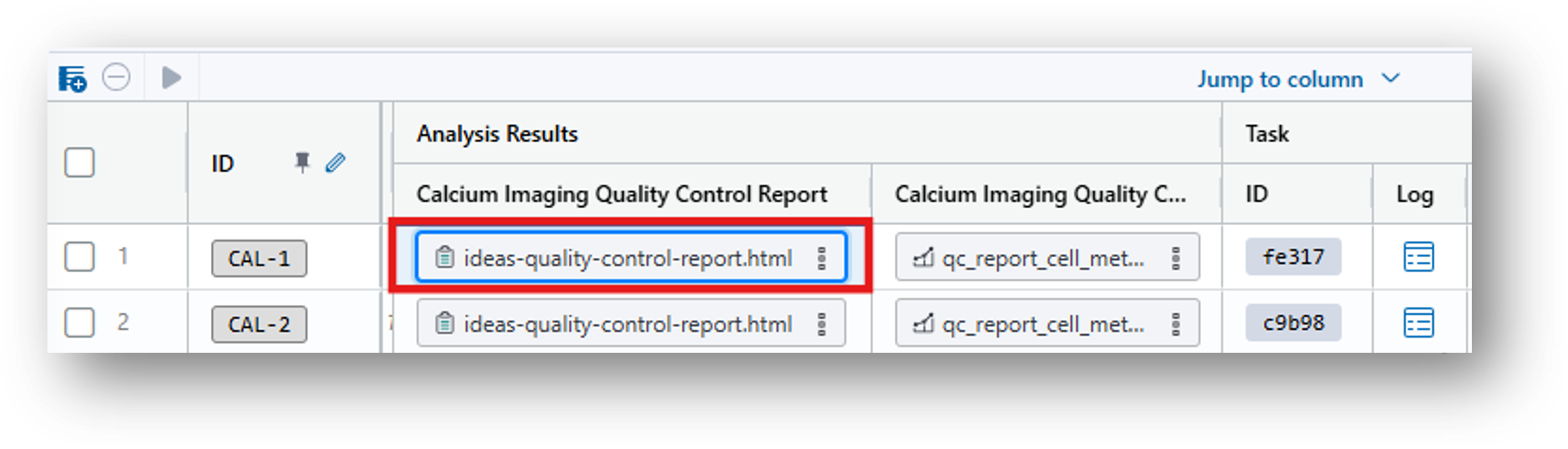
13. Once you click Create and can view the new analysis table, click and wait for the analysis to complete.
14. Scroll to the far right and select the ideas-quality-control-report.html under Analysis Results.
15. Then click  in the Preview tab to view the QC Report in your web browser. For an explanation of these results, see the documentation.
16. Similarly, you can also navigate to the Small Cohort data table to create and run a Manually Filter Cells or Automated Accept/Reject Cells Analysis Table.
- Manually Filter Cells allows users to leverage the results from the QC Report to directly select cells of interest to either accept or reject.
- Automated Accept/Reject Cells allows the user to set thresholds for automatically accepting/rejecting cells. Again, the Calcium Imaging QC Report can be leveraged to determine the best parameters/values for thresholding.
Analyze Behavioral Data
Goal
Here you’ll learn how to process and analyze behavioral recordings, including extracting tracking data and preparing it for synchronization with neural activity data.
The workflow for synchronizing behavioral and neural recordings depends on the method used for behavioral recording:
If you enabled live tracking on your nVision, then the .isxb behavioral file contains the tracking info as metadata, which can be extracted using the Extract Tracking Data from nVision Movie analysis table. However, the provided mp4 files were not tracked live, so the nVision Animal Tracking Model can calculate these metrics post hoc. This corresponds to [4] Generate/Extract tracking Data from Behavior Movie and the resulting [5] Behavior Annotations (.csv) in the IDEAS flowchart.
17. Navigate to the Small Cohort data table and create an nVision Animal Tracking Model analysis table. This uses a machine learning model to draw a bounding box around the animal for each recorded frame of the behavioral recording and calculates the approximate COM, additionally (if desired) annotating epochs during which the animal occupies designated bounding regions of interest (ROIs) within the FOV.
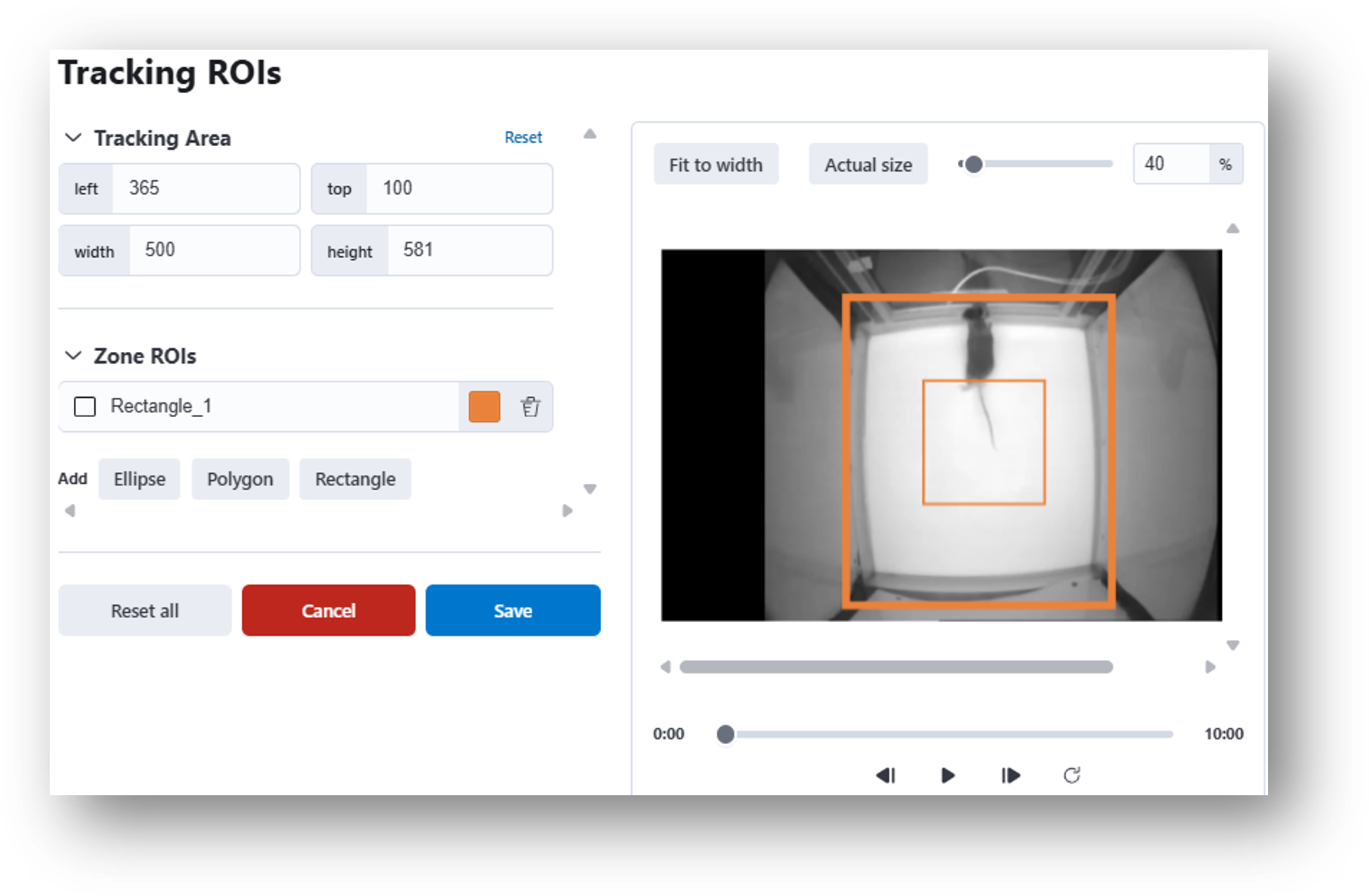
18. Select the empty rectangle under ‘Tracking ROIs’ in the nVision Animal Tracking Model analysis table and an interactive window will appear. Here you can define the overall Tracking Area or select Zone ROIs using one of the shape tools (e.g., Ellipse, Polygon, Rectangle).
19. Next you will need to constrain the Tracking Area. For these recordings, try constraining the Tracking Area by dragging the sides of the thick outer orange rectangle so they match the sides of the behavior box (see example image below).
20. Then you will need to draw Zone ROIs on the behavioral recordings. Under Zone ROIs, double click Rectangle and draw a box around the center of the arena, as in the screenshot below. Click Save. You will need to repeat these steps for both recordings. Then click .
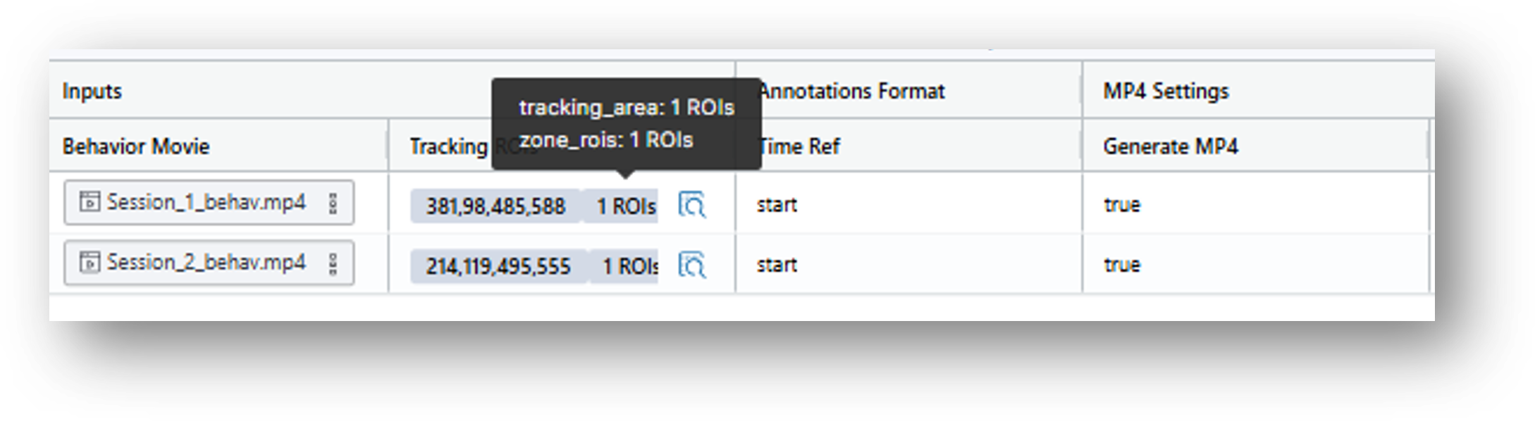
21. When you have finished, look at the nVision Animal Tracking Model Analysis table and hover over the cells in the Tracking ROI’s column to confirm that you see both the tracking_area and zone_ROIs you have defined. Then click .
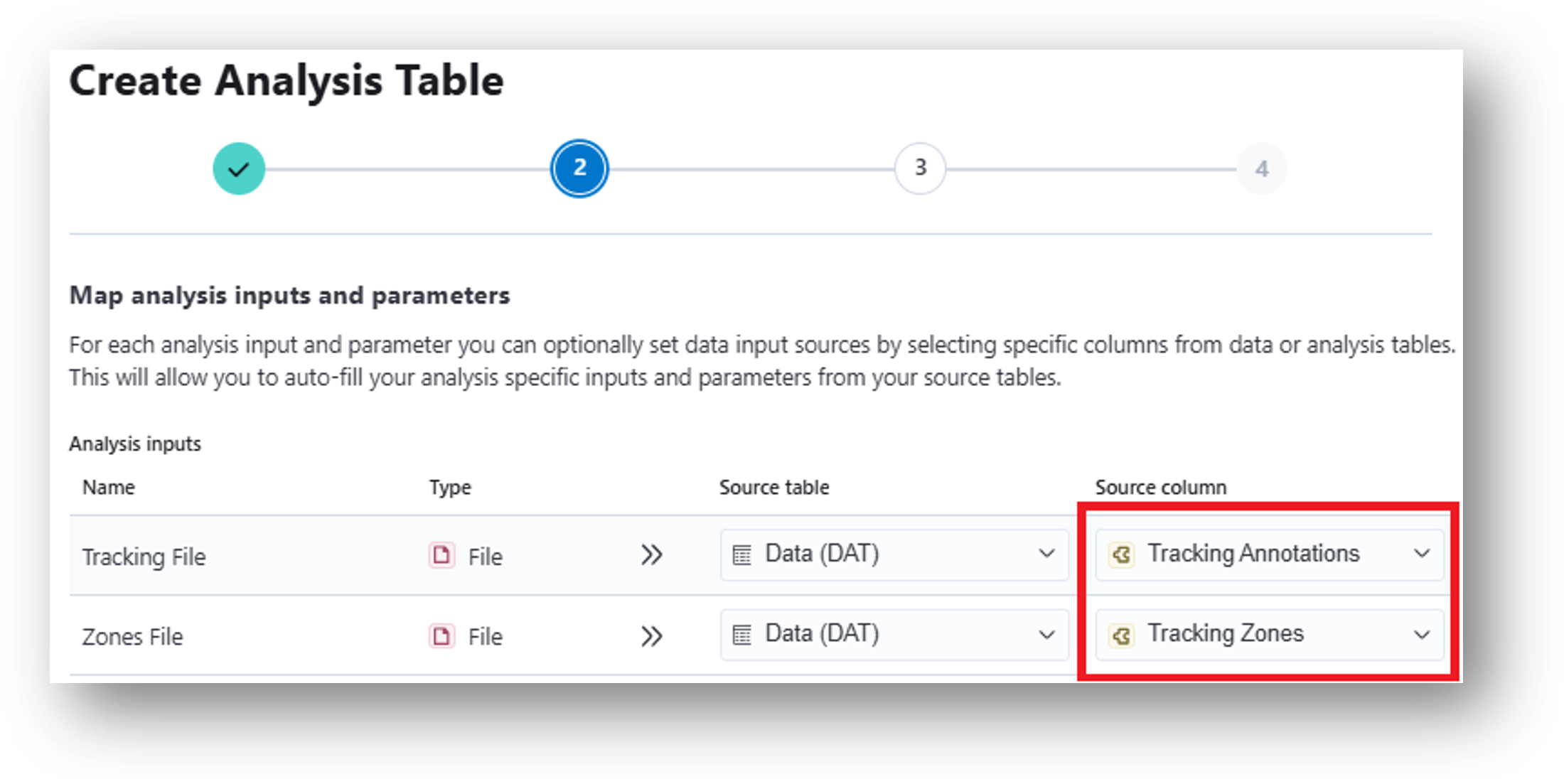
22. Input these results into the Zone Occupancy Analysis which will calculate metrics related to movement through user-defined zones (e.g., times of zone entrance/exit and epochs of zone occupancy). When mapping analysis inputs from your data table, select Tracking Annotations as your Source column for the Tracking File and Tracking Zones as your Source column for the Zones File.
23. Create table and Start All Tasks. When finished, view the three different Analysis Results at the far right of the table.
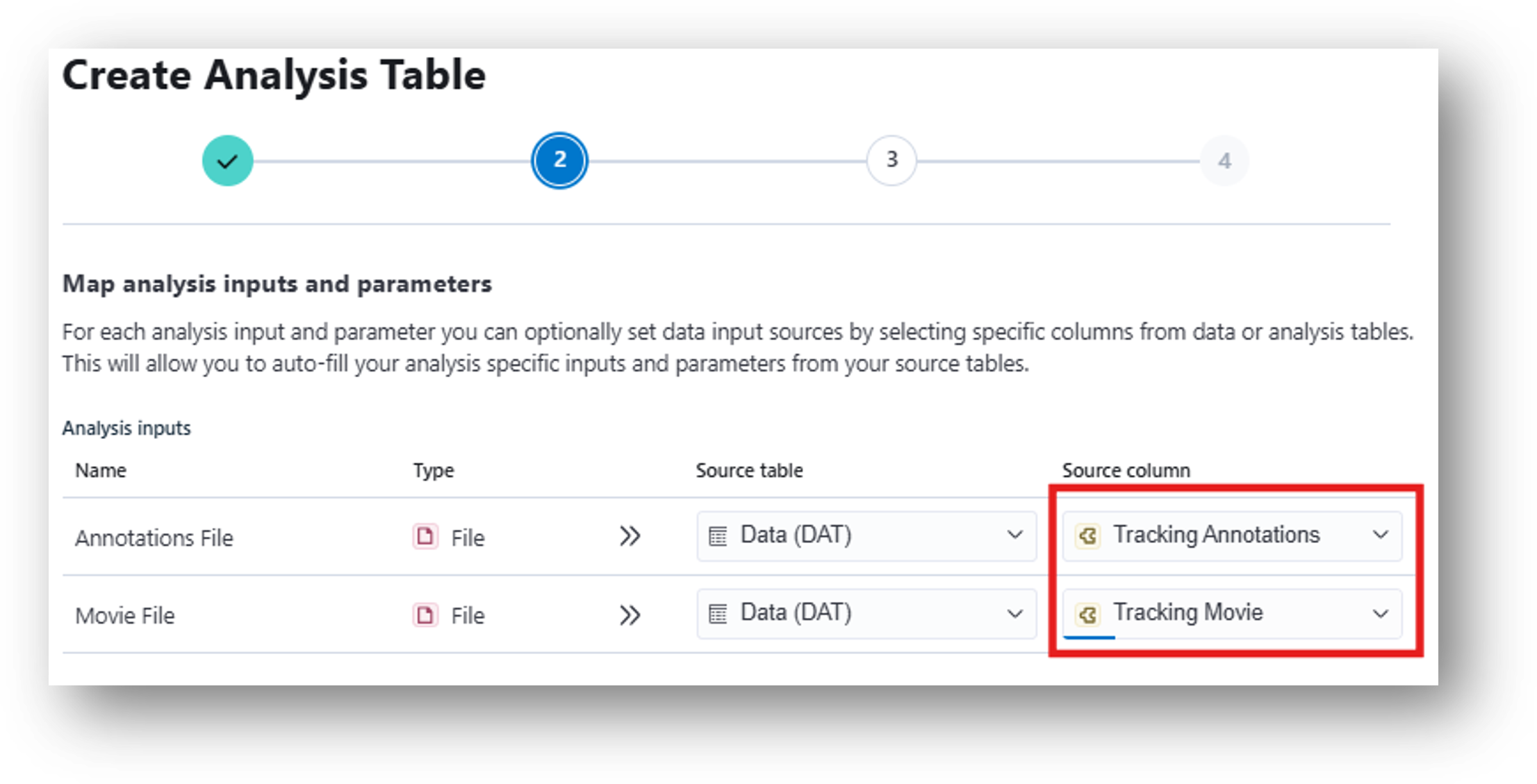
24. Then use Compute Locomotion Metrics to calculate metrics related to movement (e.g., speed, epochs of rest vs. move, etc.) This corresponds to [8] Compute Locomotion Metrics and the resulting [9] Locomotion Metrics Annotations (.csv/.pq) in the IDEAS flowchart. When mapping analysis inputs from your data table, select Tracking Annotations as your Source column for the Annotations File and Tracking Movie as your Source column for the Movie File.
25. Create the table. Under Time Column Name, replace the default value with Frame Timestamp (s). Under X Column Name and Y Column Name, enter Bounding Box Center X and Bounding Box Center Y, respectively, for each recording (note: make sure these are input exactly as shown). Start all tasks to run the table. When finished, you can view the Locomotion Metrics Analysis Results at the far right of the table.
Note
The results from the Compute Locomotion Metrics tool are expressed with the same sampling rate that was used for the behavioral recording – in this case, ~30 Hz. However, the miniscope recordings were downsampled to 10 Hz. Before performing secondary analysis on these data, it is important to synchronize the neural and behavioral inputs, such that each miniscope frame corresponds to exactly one behavior frame.
Synchronize Data
Goal
This section guides you through synchronizing your neural activity and behavioral data so you can assess how brain activity relates to behavior in your experiments.
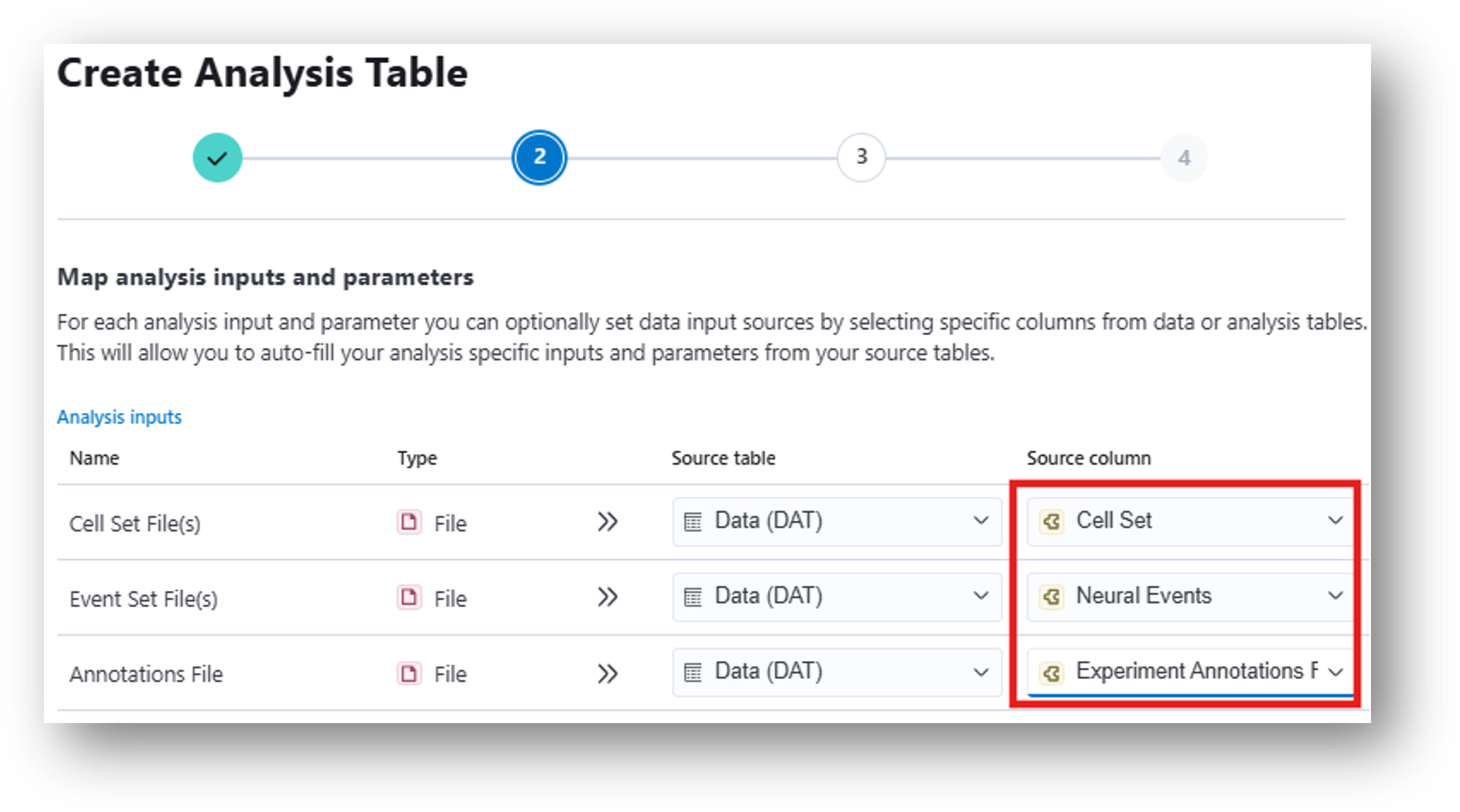
26. To synchronize the neural and behavioral inputs, the user can Insert a New Analysis from the data table and select Map Annotations to ISXD Data.
-
To choose the correct inputs from your data table, select Cell Set as the ISXD File(s) and Locomotion Metrics as the Annotation File(s).
-
Create the analysis table. Then type Frame Timestamp (s) under Time column and Zone Name under State column on your table.
Note
This will direct the analysis to synchronize behavioral time (under the heading Frame Timestamp (s)) with the neural time of the corresponding Cell Set. It will additionally label each of these frames to indicate whether the mouse was inside the rectangular ROI in the open field assay.
This analysis and the resulting neural activity-mapped parquet file correspond to [10] Map Annotations to ISXD Data and [11] Mapped Experiment Annotations (.pq) in the IDEAS flowchart.
Analyzing your Synchronized Data
Goal
Once neural and behavioral data have been synchronized, use the resulting aligned datasets to perform analyses (such as peri-event and state-based comparisons) that directly relate neural activity to specific behavioral events or states.
The following analyses correspond to steps [12] through [19] of the IDEAS flowchart.
27. Peri-event analysis (How neural signals vary before and after event timestamps)
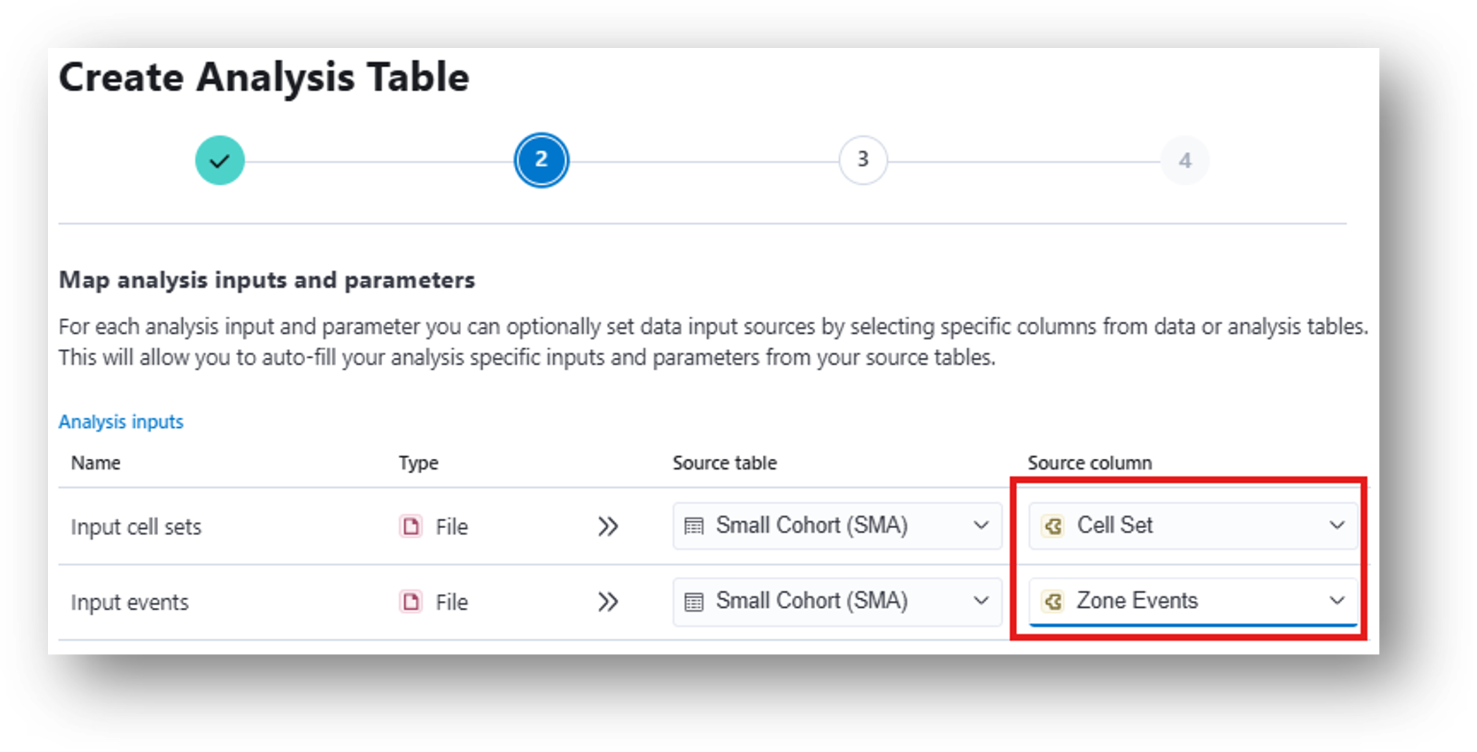
- The results from the Zone Occupancy Analysis can be used to run the Peri-event analysis, which compares neural activity pre/post annotated events. To map the correct inputs from your data table, select Cell Set for the Input cell sets row and Zone Events for the Input events row.
28. Create the table. Under Event type, enter Rectangle_1 entrance to align the neural data to timepoints where the mouse entered the rectangular ROI. You can alternately type Rectangle_1 exit if you’d prefer to analyze the data surrounding those timepoints. This corresponds to [14] Peri-Event Analysis Workflow of the IDEAS flowchart.
Once you have multiple peri-event analysis outputs, Combine and Compare Peri-Event Analysis Data will combine these for a group analysis.
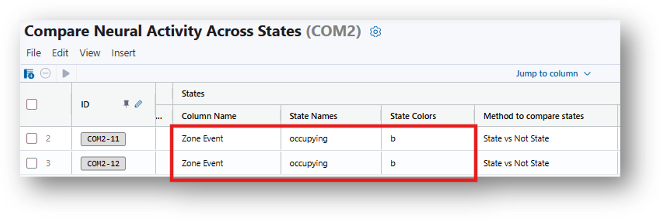
29. Run the Compare Neural Activity Across States tool (The average activity during user-specified behavioral states)
- Inputs for this analysis table are Cell Sets and Annotation Files from Zone Occupancy Analysis, Compute Locomotion Metrics, or other mapped (a.k.a. synchronized to neural movie) behavioral outputs. Finish the process and create your analysis table.
- Under Column Name, State Names, and State Colors, type Zone Event, occupying, and b respectively to specify the column of the annotation file to analyze, the state of interest - when the animal is occupying the rectangular ROI, and the color of the resulting figure.
Note
You can enter State Names of interest that correspond with the Annotations File. For instance, if you have previously run Compute Locomotion Metrics and synchronized these results with the neural recordings (using Map Annotations To ISXD Data), your states could be Rectangle_1. All other frames will be the default second state.
Note
In the event that you’ve run this analysis across multiple animals, use Combine and Compare Population Activity Data for a group analysis.
Advanced Analysis
Goal
Explore additional ways to analyze your synchronized neural activity and behavioral data.
-
Compare Neural Circuit Correlations Across States: calculates pairwise correlations between cell traces within a cell set for each specified state.
-
Compare Neural Activity Across Epochs: calculates the average activity of the calcium traces, the pairwise correlation of the calcium traces, and if an event set is provided, the average event rate during any number of user-specified epochs.