Inscopix Bottom View Mouse Pose Estimation
Compute Credits
This tool uses 2 compute credits per hour
This tool applies a pre-trained DeepLabCut model to Inscopix behavioral movies recorded from a bottom-up camera view angle.
Parameters
| Parameter Name | Description | Default |
|---|---|---|
| Input Movie File | Behavioral movie to analyze. Must be one of the following formats: .isxb, .mp4, or .avi. |
required |
| Experiment Annotations Format | The file format of the output experiment annotations file. Can be either CSV or Parquet. CSV is a more well-known file format, however Parquet is recommended because it's proven to be more performant in terms of runtime, and space efficiency. Read more about the parquet file format here. |
Parquet |
| Crop Rectangle | Coordinates of the crop rectangle applied to the movie FOV prior to running the model. It is strongly advised to focus analysis on the arena, as model inference will run faster (convolutions over a smaller area) and predictions will be of higher quality (no erroneous labeling of out-of-arena elements). Formatted as a comma-separated list of 4 integers in the following order: x_left, x_right, y_top, y_bottom. If None, then no cropping is applied. |
None |
| Window Length | Length of the median filter (in units of number of frames) applied to the predictions. Must be an odd integer. If set to 1, then no filtering is performed. |
5 |
| Displayed Body Parts | List of body parts to plot in the output video. If all, then all 8 body parts are plotted. Otherwise a comma-separated list of strings selects a subset of body parts to plot, e.g., nose, neck. The body parts available for plotting are: nose, neck, L_fore, R_fore, L_hind, R_hind, tail_base, tail_tip. |
all |
| P Cutoff | Cutoff threshold (in likelihood) for predictions when labelling the input movie. Predicted body part coordinates with likelihood below the p-cutoff threshold are not displayed. Must be a float between [0, 1). | 0.6 |
| Dot Size | Size in pixels to draw a point labelling a body part. | 5 |
| Color Map | Color map used to color body part labels. Any matplotlib colormap name is acceptable. | rainbow |
| Keypoints Only | Only display keypoints (i.e., body part predicted labels) in the output video, not input video frames. | false |
| Output Frame Rate | Positive number, output frame rate for labeled video. If None, use the input movie frame rate. | None |
| Draw Skeleton | If True adds a line connecting the body parts, making a skeleton on each frame. Colors of the body part labels and their connecting lines are specified by the Color Map. | false |
| Trail Points | Number of past labels to plot in a frame, or trail length (for displaying history). | 0 |
Description
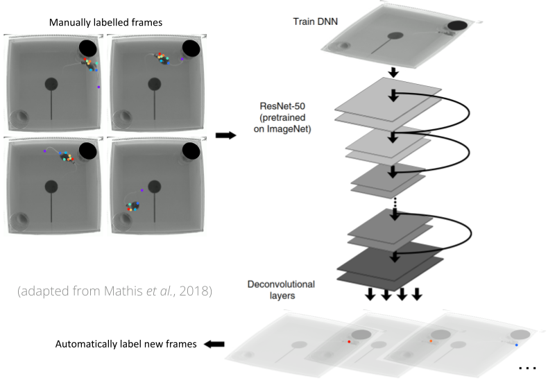
This tool employs a pre-trained convolutional deep neural network model for pose estimation. The pre-trained model that is executed by the tool was trained using DeepLabCut, an open-source library for pose estimation using deep learning. The version of DeepLabCut used by the tool is version 2.3.0. The following figure shows an example of the structure of the model.
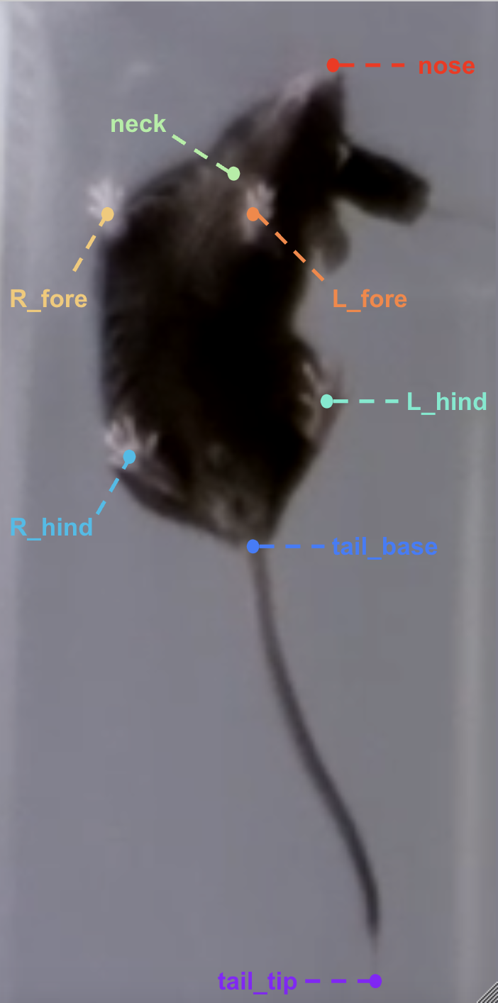
The pre-trained model tracks 8 different body parts of a mouse (nose, neck, left forepaw, right forepaw, left hindpaw, right hindpaw, tail base, and tailtip), as illustrated in the figure below.
The tool executes the following three main steps using DeepLabCut.
- Analyze videos: Run the pre-trained model on an input movie. This calls the function
analyze_videosin thedeeplabcutAPI. - Filter predictions: Filter the model predictions in order to remove outliers. This calls the function
filterpredictionsin thedeeplabcutAPI. - Label video: Label the input movie with the filtered predictions. This calls the function
create_labeled_videoin thedeeplabcutAPI.
How this model was trained
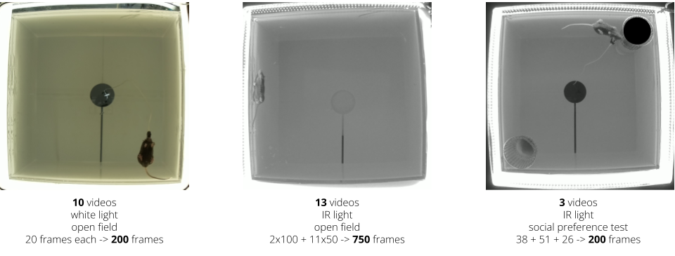
In order to generalize well across different behavioral movies, the model was trained across a number of bottom view movies with different lighting conditions and environments. The following table summarizes the types of movies that were used to train the model.
| Lighting Condition | Arena/Environment | Number of Movies | Number of Frames (overall) |
|---|---|---|---|
| White Light | Open Field | 10 | 200 |
| IR Light | Open Field | 13 | 750 |
| IR Light | Social Preference Test | 3 | 115 |
Overall, the model was trained on a total of 26 movies, 1065 frames, across 2 lighting conditions and 2 arenas/environments. The figure below shows examples of these different types of movies.
In addition, data augmentation was used (imgaug) to extend further model generalization, e.g., to black and white movies and to a range of mouse sizes and image contrast and sharpness.
The model was trained over 1000000 iterations, and the snapshot (model coefficients) minimizing the test set error was selected (min. error of 5.07 pixels at 420000 iterations).
Outputs
This model produces three different outputs. Each output corresponds to a step that is executed by the tool.
Pose Estimates H5 File
An .h5 file containing the model predictions.
The predictions are stored as a MultiIndex Pandas Array.
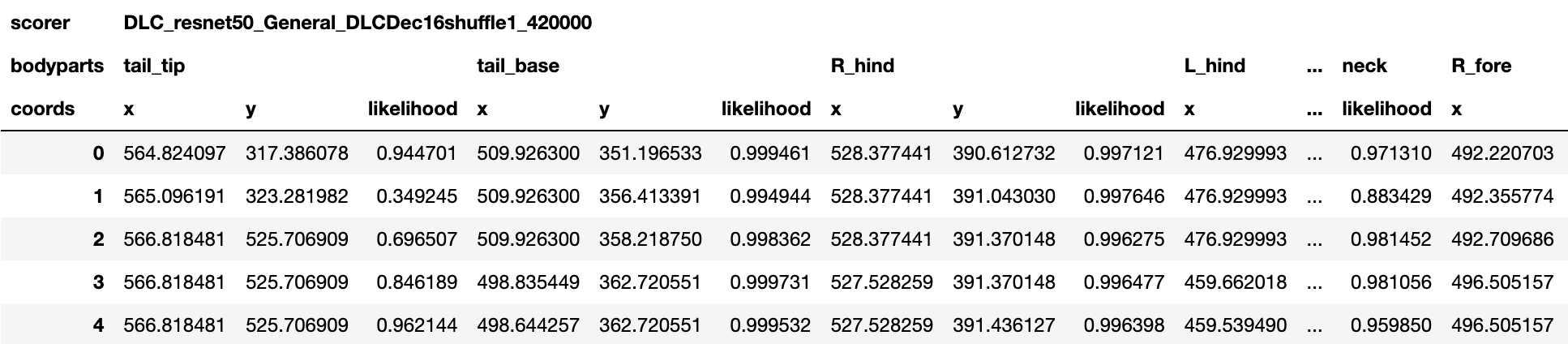
The files contains the name of the network, body part name, (x, y) label position in pixels, and the likelihood (i.e., how confident the model was to place the body part label at those coordinates) for each frame per body part.
The following figure shows an example of this output.
If the Window Length parameter is set to one, then no filtering is performed and the raw pose estimates (aka coordinates or keypoints) are output. Otherwise if the Window Length is greater than one, then filtering is performed and the filtered pose estimates are output.
Experiment Annotations File
The pose estimates in IDEAS experiment annotations format. This can be either a .csv or .parquet file depending on the Experiment Annotations Format parameter. The following figure shows an example of this output. Note: Only a subset of the model body parts are shown in the figure.
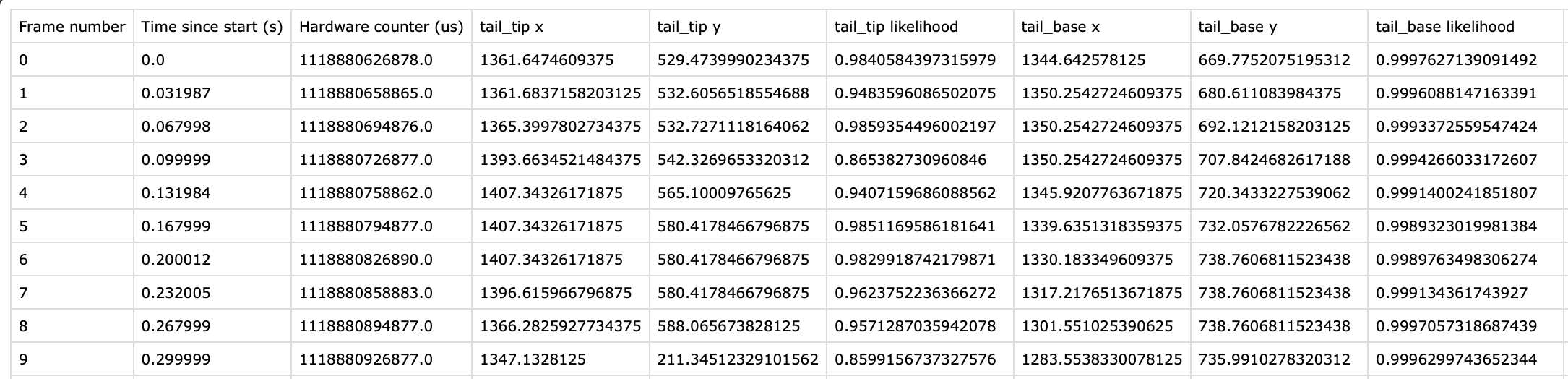
For every body part estimated by the model, there are three columns that are output: x, y, and likelihood. In addition, there is a Frame Number column in the output labeling every frame of the input movie analyzed. There are also two columns containing timestamps:
Time since start (s): Timestamp in seconds for every frame of the input movie, relative to the start of the movie.Hardware counter (us): Only included for.isxbinput movies. This column contains the hardware counter timestamps in microseconds for every frame of the input movie. These are the hardware counter values generated by the nVision system which can be compared to corresponding hardware counter values in.isxd,.gpio, and.imufiles from the same synchronized recording. These timestamps will be used downstream in theMap Annotations to ISXD Datatool in order map frames from annotations to isxd data, so the two datasets can be compared for analysis.
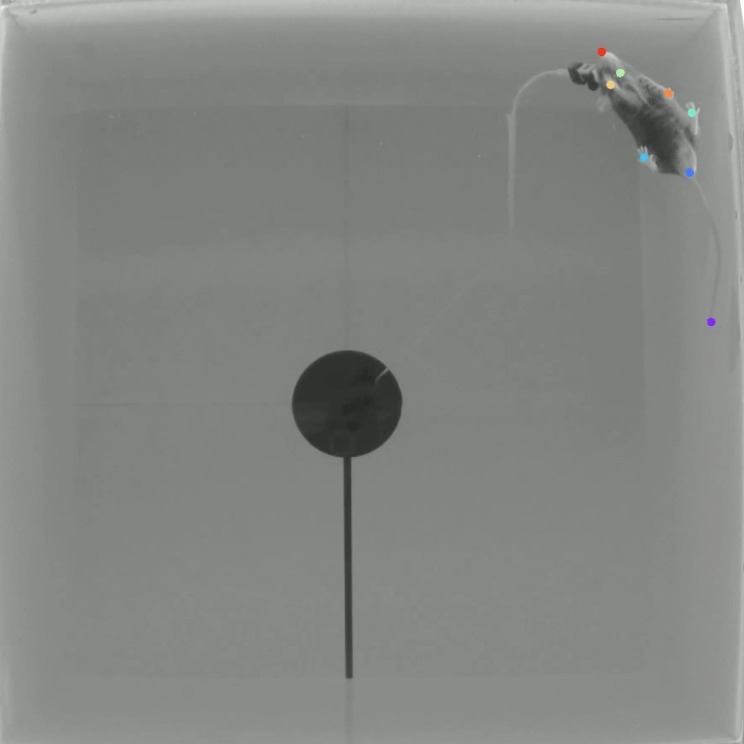
Labeled MP4 File (for visualization)
A .mp4 file containing the model predictions annotated on every frame of the input movie.
The following figure shows an example of this output.
Next Steps
Here are some examples of subsequent analyses that can be executed using the outputs of this tool:
- Average DeepLabCut Keypoints: Average the keypoint estimates in each frame of the tool output, and use this to represent the mouse center of mass (COM).
- Compute Locomotion Metrics: Compute instantaneous speed and label states of rest and movement from averaged keypoints.
- Compare Neural Activity Across States: Compute population activity during states of rest and movement from locomotion metrics.
- Compare Neural Circuit Correlations Across States: Compute correlations of cell activity during states of rest and movement from locomotion metrics.
- Combine and Compare Population Activity Data: Combine and compare population activity from multiple recordings and compare across states of rest and movement.
- Combine and Compare Correlation Data: Combine and compare correlations data from multiple recordings and compare across states of rest and movement.