PCA-ICA¶

This tool uses 1.0 compute credits per hour.

PCA-ICA is used to identify signals from independent components (ICs) in movie data. These signals correspond to spatial filter images, which define where the components are, and temporal traces, which define when the components are active. Ideally, each component is an in-focus neural soma, but we may also expect to identify some confounding components that may be out-of-focus somata, non-somatic, or non-biological signals as illustrated in this figure.

We assume that movie data contains components that are both spatially and temporally defined. Some of these components may correspond to neural somata, while others may not. There may also be some spatial overlap between the components. Here, we present a synthetic example that captures these properties:

Inputs¶

Parameter	Required?	Default	Description
Input Movies Files	True	N/A	path to the input isxd movie files
Number of PCs	True	150	The number of principal components (PCs) to estimate.
Number of ICs	True	120	The number of independent components (ICs) to estimate.
Unmixing Type	True	spatial	Type of unmixing that needs to be applied. Can be either “temporal”, “spatial” or “spatio-temoporal”
ICA Temporal Weight	True	0	The temporal weighting factor used for ICA.
Maximum Iterations	True	100	The maximum number of iterations for ICA
Convergence Threshold	True	1e-05	The convergence threshold for ICA.
Block Size	True	1000	The size of the blocks for the PCA step. The larger the block size, the more memory that will be used.
Auto Estimate Number of ICs	True	True	If True the number of ICs will be automatically estimated during processing. The number of PCs will be overriden and set to 1.2 times the number of estimated ICs.
Average Cell Diameter	True	10	Average cell diameter in pixels (only used when auto_estimate_num_ics is set to True)

File Inputs¶

Source Parameter	File Type	File Format
Input Movies Files	miniscope_movie, miniscope_movie	isxd, isxc

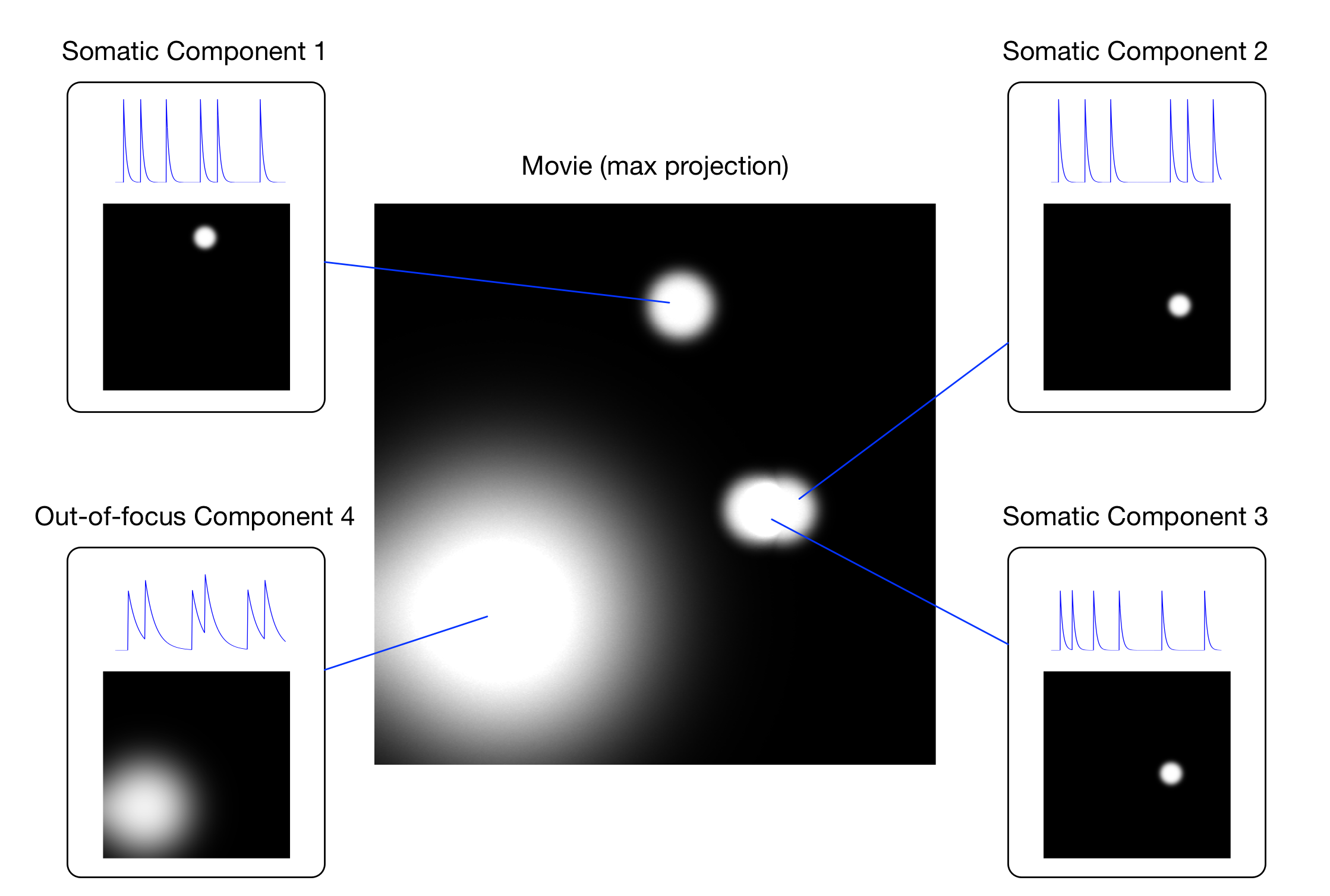
Figure: Components of the movie

Component 1 is somatic and does not spatially overlap with any other component; components 2 and 3 are somatic, but spatially overlap; component 4 is an out-of-focus soma.

We may also expect that some of the components have some spatial overlap. This means that performing a basic ROI analysis with manualRois is not advisable (this figure).

In order to identify these images and traces, PCA-ICA performs many processing steps that are summarized below.

movieMatrix. The movie frames are rasterized into 1D vectors and stacked into a 2D matrix.
meanSubtractions. The mean image and mean trace are subtracted from the movie matrix.
Principal Component Analysis. The movie matrix is decomposed into principal image and trace components in order to reduce dimensionality and precondition the data.
Standard Deviation Normalization. The principal image and trace components are normalized so that their standard deviation is one.
spatiotemporalMixing. The principal image and trace components are weighted and combined to form the input data for ICA.
ica. An unmixing matrix is found that unmixes the principal components to give the independent components that maximize skewness.
unmixing. The unmixing matrix is applied to the principal image and/or trace components to give independent image and trace components.

These steps are mostly inspired by the dynamic calcium imaging data processing in ¹. The purpose of this document is to describe these steps in more detail.

The Movie Matrix¶

A movie is naturally thought of as a sequence of frames (images). For each of those images, we can rasterize the 2-dimensional image into a 1-dimensional vector as illustrated in the following figure.

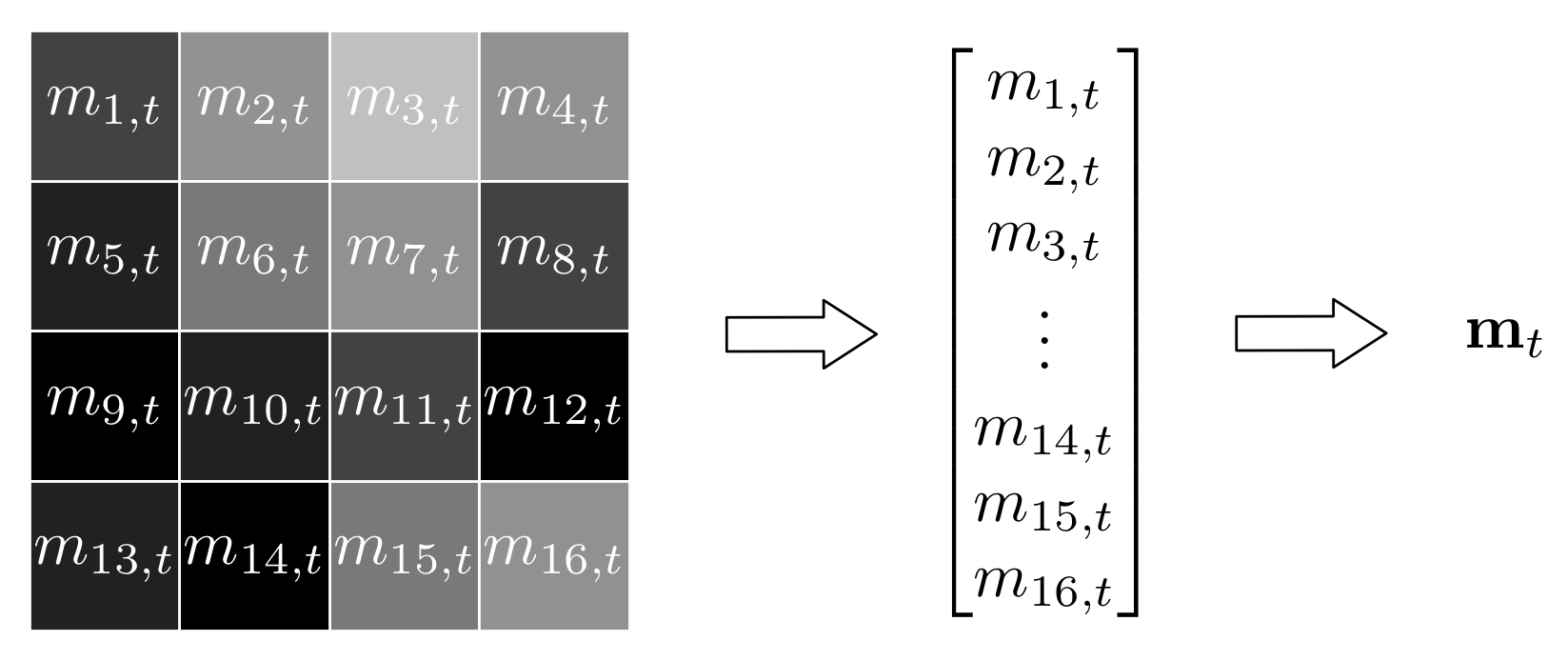
Figure: Frame rasterization

A single frame of the movie can be rasterized into a 1-dimensional vector by scanning the image matrix by row and stacking the values into the vector. Here, a frame with four rows and four columns is rasterized into a vector with sixteen elements

If we do this for all frames in a movie, we can stack the resulting vectors into a matrix. More formally, the movie matrix is written using the following mathematical notation:

\[ \mathbf{M}=\begin{bmatrix}\mathbf{m}_1 & \mathbf{m}_2 & ... & \mathbf{m}_T\end{bmatrix} \]

where $\mathbf{M}$ is the $N \times T$ movie matrix, $N$ is the number of pixels in one frame, $T$ is the number of frames, and $\mathbf{m}_t$ is frame number $t$,

This algorithm assumes that the movie data can be approximately decomposed into a Number of ICs, which we denote as $C$, each with an associated rasterized spatial image $\mathbf{s}_c$ and an activity trace $\mathbf{a}_c$.

In this example, we know that there are $C = 4$ components as illustrated in the figure below.

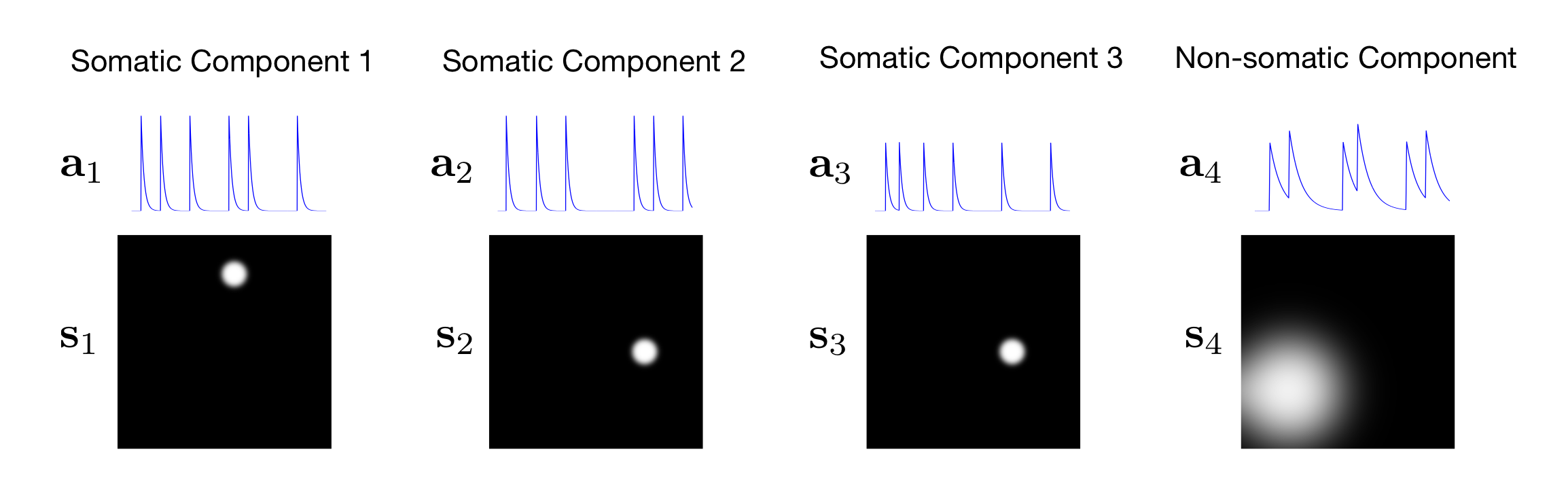
Figure: Movie Components

For each component $c$, we let $\mathbf{s}_c$ represent the rasterized image and let $\mathbf{a}_c$ represent the trace.

To approximate one frame of the original movie, the algorithm sums over all component images and weights them according to their corresponding trace values at that time, as illustrated in this figure.

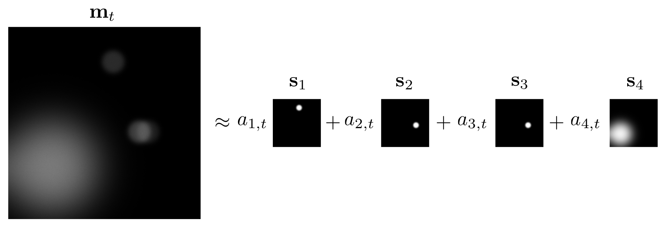
Figure: Frame Decomposition

The algorithm assumes that one frame of the movie can be approximated by summing the contributions from image components weighted by the corresponding trace component values at that frame index.

In the same way we rasterized the movie frames, we can also rasterize all the spatial images of the components to form an $N \times C$ matrix $\mathbf{S}$:

\[ \mathbf{S} = \begin{bmatrix} \mathbf{s}_1 & \mathbf{s}_2 & \dots & \mathbf{s}_C \end{bmatrix} \]

where $\mathbf{s}_c$ is the spatial image of component $c$.

Similarly, we can stack the activity traces into a $T \times C$ matrix $\mathbf{A}$:

\[ \mathbf{A} =\begin{bmatrix}\mathbf{a}_1 & \mathbf{a}_2 & \dots & \mathbf{a}_C\end{bmatrix} \]

Now we can summarize this approximate decomposition of the movie formally as:

\[ \begin{bmatrix} \mathbf{m}_1 \mathbf{m}_2 ... \mathbf{m}_T \end{bmatrix} \approx \begin{bmatrix} \mathbf{s}_1 \mathbf{s}_2 \dots \mathbf{s}_C \end{bmatrix} \begin{bmatrix} \mathbf{a}_1^\top \\ \mathbf{a}_2^\top \\ \dots \\ \mathbf{a}_C^\top \end{bmatrix} \]

\[ \mathbf{M}\approx \mathbf{S} \, \mathbf{A}^\top. \]

It is important to note that while the movie $\mathbf{M}$ is known, both the images $\mathbf{S}$ and the traces $\mathbf{A}$ are unknown and must be estimated. In combination, PCA and ICA provide these estimates.

Mean Subtractions¶

Internally, PCA-ICA subtracts both the mean image and the mean trace from the original movie matrix $\mathbf{M}$. It does this for two reasons. The first is that PCA requires one of these to be subtracted from the movie data. The second is that the ICA algorithm we use requires zero-mean data, and, in general, that data is a mixture of spatial and temporal principal components extracted from the movie in pca.

More formally, we can form a zero-mean $N \times T$ matrix $\mathbf{M}$ where:

\[ m'_{nt} = m_{nt} - \bar{s}_n - \bar{a}_t \]

where $\bar{s}_n$ is the empirical mean image of the movie evaluated at pixel $n$:

\[ \bar{s}_n = \frac{1}{T} \sum_{t=1}^T m_{nt} \]

and $\bar{a}_t$ is the empirical mean trace of the movie evaluated at time point $t$:

\[ \bar{a}_t = \frac{1}{N} \sum_{n=1}^N m_{nt} - \bar{s}_n. \]

This means that for each pixel, the corresponding mean pixel value over time is calculated and this is subtracted from that pixel value in every frame of the movie. The mean trace is then subtracted from the resulting movie. This means that the average pixel value for each frame is calculated, then subtracted from all pixels in that frame to produce a new modified movie $\mathbf{M}$.

This modified movie is what is further processed in this algorithm. Note that the mean trace subtraction step will compensate for any gradual signal changes over time, such as those caused by photobleaching or LED power fluctuations.

Principal Component Analysis¶

Initially, our $N \times T$ movie matrix $\mathbf{M}$ is likely to be large. Using the standard processing workflow on a typical set of recordings, the number of pixels will be approximately $N = 500 \times 500 = 2.5 \times 10^5$ and the number of time points will be approximately $T = 5 \times 10^4$.

The goal of PCA is to compress the large movie matrix into a smaller matrix that can be processed more easily by ICA. During the compression process, PCA also removes some noise from the movie data, which helps ICA find a better solution. The Number of PCs, which we denote as $K$, controls the size of one of the dimensions of that smaller matrix.

PCA assumes that the movie matrix can be approximately decomposed into a special set of matrices with some particular properties. This is known as the truncated or low rank singular value decomposition of the matrix. Formally, we can write:

\[ \mathbf{M} \approx \mathbf{U} \mathbf{\Sigma} \mathbf{V}^\top \]

where $\mathbf{U}$ is an $N \times K$ matrix that contains a set of $K$ principal image components:

\[ \mathbf{U} = \begin{bmatrix} \mathbf{u}_1 & \mathbf{u}_2 & \dots & \mathbf{u}_K \end{bmatrix}. \]

$\mathbf{V}$ is a $T \times K$ matrix that contains a set of $K$ principal trace components:

\[ \mathbf{V} = \begin{bmatrix} \mathbf{v}_1 & \mathbf{v}_2 & \dots & \mathbf{v}_K \end{bmatrix} \]

and $\mathbf{\Sigma}$ is a diagonal matrix that contains a set of $K$ scalar, or singular, values:

\[ \mathbf{\Sigma} = \begin{bmatrix} \sigma_1 & 0 & \dots & 0 \\ 0 & \sigma_2 & \dots & 0 \\ \vdots & \vdots & \ddots & \vdots \\ 0 & 0 & \dots & \sigma_K \end{bmatrix}. \]

The images and traces are special because they are mutually orthogonal and unitary:

\[ \mathbf{U}^\top \mathbf{U} = \mathbf{I} \\ \mathbf{V}^\top \mathbf{V} = \mathbf{I}, \]

and the scalar values are special because they are positive and non-increasing:

\[ \sigma_k > 0 \quad \forall k \\ \sigma_{k} \geq \sigma{k+1} \quad k = 1 \dots K-1. \]

The number of PCs $K$ is typically chosen to be much less than the minimum of $Nand $T to achieve the desired compression. If $\sigma_K$ is very close to zero, the algorithm will reduce $K$ to remove these degenerate components. As a result, we know that $\mathbf{U}$ and $\mathbf{V}$ have rank $K$.

In a sense, PCA already provides a solution to our original spatiotemporal decomposition problem. The matrix $\mathbf{U}$ describes the spatial images of the components, and the matrix product $\mathbf{V} \mathbf{\Sigma}$ describes the corresponding activity traces. However, these components may contain mixtures of the original components, as illustrated in the figure below.

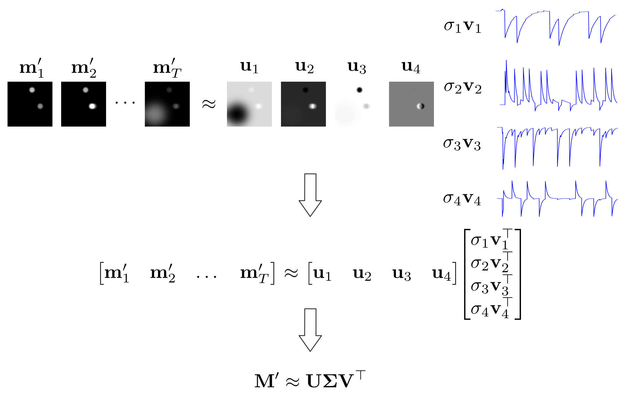
Figure: Movie SVD

PCA provides one way to approximately decompose the movie matrix into a set of image and trace components. Using this example, we can see that images and traces may be negated, which can be corrected, but may also contain mixtures of the independent components.

One way to consider $\mathbf{U}$ is as a matrix containing $N$ samples of $K$ random variables. The empirical mean of each random variable will be zero because of the mean subtractions. Note that the empirical variance of each random variable will be equal to $\frac{1}{N - 1}$ because each principal component is unitary. Similarly, we can consider $\mathbf{V}$ to be a matrix containing $T$ samples of $K$ random variables, each with an empirical mean of zero and an empirical variance of $\frac{1}{T - 1}$.

The skewness of each random variable is more interesting. It will roughly depend on how many more large positive values there are than large negative values. For example, as illustrated in this figure, we can view the empirical distributions of $\mathbf{u}_3$ and $\mathbf{v}_3$ from our running synthetic example.

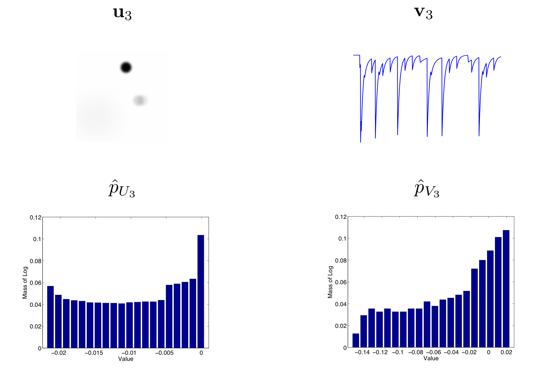
Figure: Principal Component Distributions

Here we show the third principal image and trace components and their corresponding empirical distributions. In order to highlight the skewness of the distribution, we use the normalized log histogram $\hat{p}$ for the empirical distribution.

In the example above, the skewness of both the image and trace distributions are negative. For a neural soma, the image component ideally contains many low values, which should represent the background, and a small number of high values, which should represent the cell body. This should result in positive skew. We may also expect the trace to be similarly distributed, but this will depend on how active that component is.

Standard Deviation Normalization¶

The principal image and trace components are normalized so that the empirical standard deviation of each component vector is one. This is performed in order to make the ICA algorithm more simple and efficient.

More formally, we can write the normalized image components as:

\[ \mathbf{u}'_{k} = \sqrt{N - 1} \mathbf{u}_k \]

and the normalized trace components as:

\[ \mathbf{v}'_{k} = \sqrt{T - 1} \mathbf{v}_k. \]

Note that the normalization is simple because the $\mathbf{u}_k$ and $\mathbf{v}_k$ are already zero-mean, due to the mean subtractions, and also have unit norm due to the singular value decomposition used for PCA.

Spatiotemporal Mixing¶

The weight of temporal information in spatio-temporal ICA (0 to 1) setting, which we also denote as $\mu$, was introduced in ¹. It allows a mix of the principal image and trace components to be used as input to the ICA algorithm.

Choosing an appropriate value of $\mu$ will depend on several factors. These include the number of cells, number of pixels, and number of time frames. However, the study in ¹ concluded that a choice between 0 and 0.5 for the value of $\mu$ often yields the best reconstruction of cell-like ICs (see Supplementary Figure 3 in ¹ ) . The default value is 0 because this gives good empirical performance and is theoretically easy to explain.

If $\mu = 0$, the algorithm ignores temporal information, i.e. only uses the principal image components from PCA as input for ICA:

\[ \mathbf{Y} = \mathbf{U}. \]

If $\mu = 1$, the algorithm ignores spatial information, i.e. only uses the principal trace components from PCA as input for ICA:

\[ \mathbf{Y} = \mathbf{V}. \]

If $\mu \in (0, 1)$, the algorithm uses both spatial and temporal information by combining the principal image and trace components from PCA as input for ICA. This combination is performed by weighting the components and stacking the matrices of images and traces on top of each other:

\[ \mathbf{Y} = \begin{bmatrix} (1 - \mu) \mathbf{U}' \\ \mu \mathbf{V}' \end{bmatrix} \]

Note that this is a legal operation because both $\mathbf{U}'$ and $\mathbf{V}'$ have $K$ columns.

Independent Component Analysis¶

In general, ICA is an algorithm used to solve blind source signal separation problems. In our case, the source signals correspond to the desired image and trace components. ICA assumes that these source signals are independent and are mixed to produce observed data where the source signals are not easily identifiable. Using our notation, the independent source images are stored in the matrix $\mathbf{S}$ and the independent source traces are stored in the matrix $\mathbf{A}$. In this sense, ICA provides a solution to the movie matrix decomposition problem stated above.

ICA assumes the input data is a mixed version of the underlying independent components. First, as was done for the input principal components, we stack the independent image and trace components into a combined matrix of independent components $\mathbf{X}$. More formally, we have:

\[ \mathbf{X} = \begin{bmatrix} \mathbf{S}' \\ \mathbf{A}' \end{bmatrix} \]

where $\mathbf{S}'$ contains the underlying independent component images and where $\mathbf{A}'$ contains the independent component traces, which may be different from the actual component images $\mathbf{S}$ and traces $\mathbf{A}$.

ICA finds an unmixing matrix $\mathbf{F}$ that separates the independent components from the input data:

\[ \mathbf{X} = \mathbf{Y} \mathbf{F} \]

where $\mathbf{F}$ is a $K \times C$ unmixing matrix:

\[ \mathbf{F}= \begin{bmatrix} \mathbf{f}_1 & \mathbf{f}_2 & ... & \mathbf{f}_C \end{bmatrix}. \]

Given the linear relationship between $\mathbf{X}$ and $\mathbf{Y}$, and that $\mathbf{F}$ is an unknown fixed parameter, the randomness of $\mathbf{Y}$ implies that $\mathbf{X}$ stores $N + Tsamples of $C random variables.

More formally, one sample of the random variable $X_c$ is drawn from a probability distribution:

\[ x_{n,c} \sim p_{x_{c}}(x_{n,c}) \quad \forall c \in \{1, \dots, C\} \, \forall n \in \{1, \dots, N + T\}. \]

Independence implies lack of correlation, which means that the independent components are uncorrelated. Because the columns of $\mathbf{X}$ are zero-mean, they are mutually orthogonal:

\[ \sum_{n=1}^{N+T} x_{n,c} x_{n,c'} = 0 \quad \forall c \neq c'. \]

Because the columns of $\mathbf{Y}$ are mutually orthogonal (they consist of stacked, scaled principal components), the columns of $\mathbf{F}$ must also be mutually orthogonal:

\[ \mathbf{F}^\top \mathbf{F} = \mathbf{I}. \]

In this sense, the independent components are found by projecting the principal components onto a new set of orthogonal bases defined by the columns of $\mathbf{F}$. If the number of principal components $K$ is equal to the number of independent components $C$, then $\mathbf{F}$ is a square orthogonal matrix and thus rotates and flips the principal components. The figure below summarizes the linear model assumption of ICA.

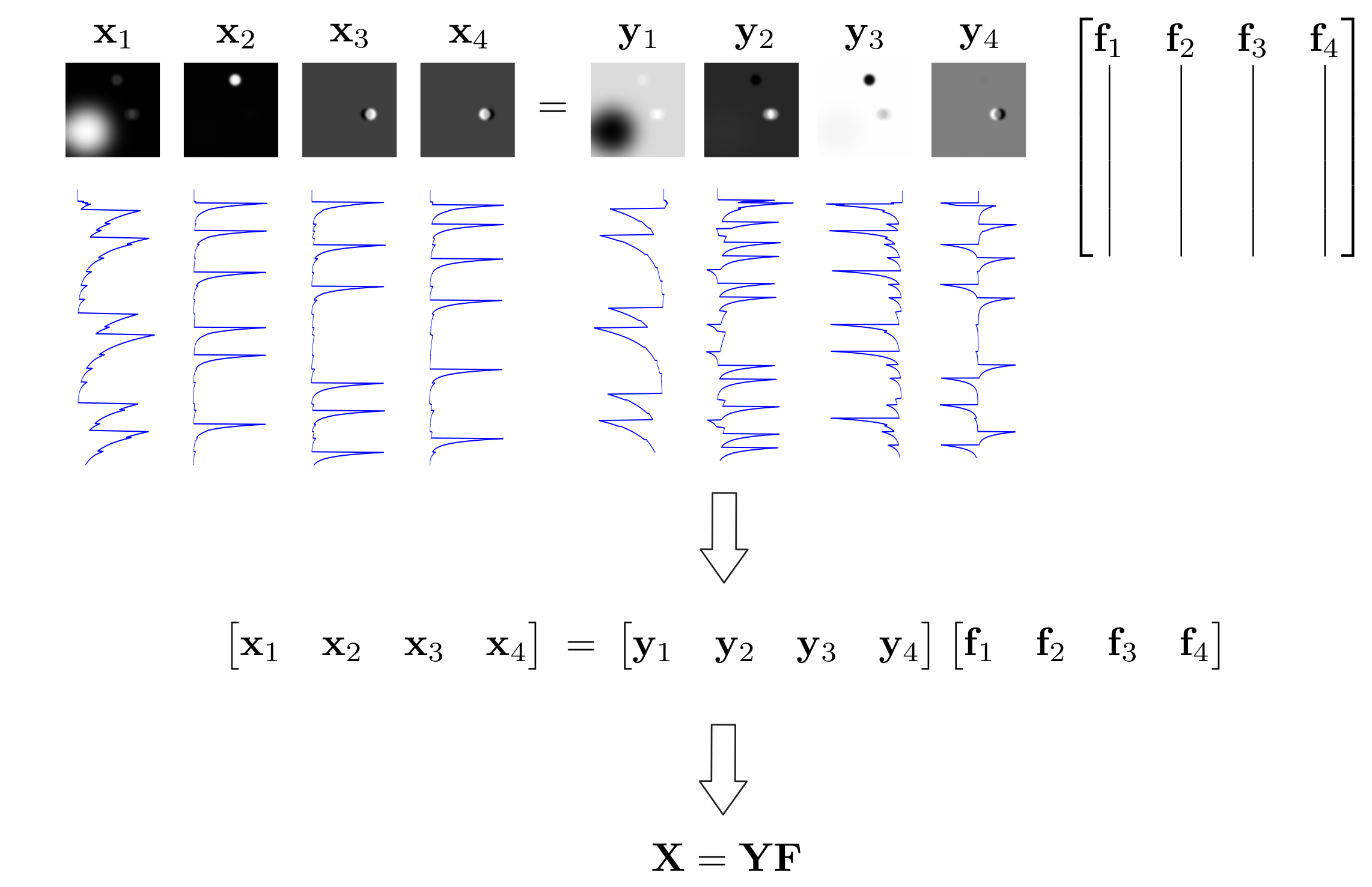
Figure: ICA Model

Our ICA model assumes that the independent components $\mathbf{X}$ are the result of projecting the observed principal components $\mathbf{Y}$ onto a new set of orthogonal bases defined by the columns of $\mathbf{F}$.

As previously motivated by this figure, we want to transform the compressed data obtained from PCA, $\mathbf{Y}$, so that we maximize the skewness of the resulting distributions. The ICA algorithm we use attempts to find the unmixing matrix $\mathbf{F}$ that produces the independent components $\mathbf{X}$ with maximal skewness, under the constraint that the columns of $\mathbf{F}$ are orthogonal.

More formally, we want to solve the following optimization problem:

\[ \hat{\mathbf{F}}= \underset{ \mathbf{F} \, \mathrm{s.t.} \mathbf{F}^\top \mathbf{F} = \mathbf{I} }{ \mathrm{argmax} } \left[ \sum_{c=1}^C \mathbb{E}_{p_{x_c}} \left[ x_c^3 \right] \right] \]

\[ =\underset{ \mathbf{F} \, \mathrm{s.t.} \mathbf{F}^\top \mathbf{F} = \mathbf{I} }{ \mathrm{argmax} } \left[ \sum_{c=1}^C \mathbb{E}_{p_{x_c}} \left[ (\mathbf{y} \mathbf{f}_c)^3 \right] \right]. \]

This constrained optimization problem is difficult because it is defined with respect to the entire matrix $\mathbf{F}$. In our method, we relax the constraint by assuming that the columns of $\mathbf{F}$ are unitary and iterate between solving the following problem:

\[ \hat{\mathbf{F}}= \underset{ \mathbf{F} \, \mathrm{s.t.} || \mathbf{f}_c ||^2 = 1 \, \forall c }{ \mathrm{argmax} } \left[ \sum_{c=1}^C \mathbb{E}_{p_{x_c}} \left[ (\mathbf{y} \mathbf{f}_c)^3 \right] \right] \]

and projecting the resulting $\hat{\mathbf{F}}$ onto the constrained space defined by $\mathbf{F}^\top \mathbf{F} = \mathbf{I}$.

This iterative procedure is stopped either when we reach the ICA Max Iterations settings value or when the fractional change in the solutions from two consecutive iterations falls below the ICA Convergence Threshold settings value.

An example of a pair of image and trace independent components from ICA and their empirical distributions are shown in this figure. These should be compared with the pair of image and trace principal components shown in this figure and the underlying ground truth components shown in this figure. Note that the independent components have higher skewness than the principal components and are also much closer to the ground truth components.

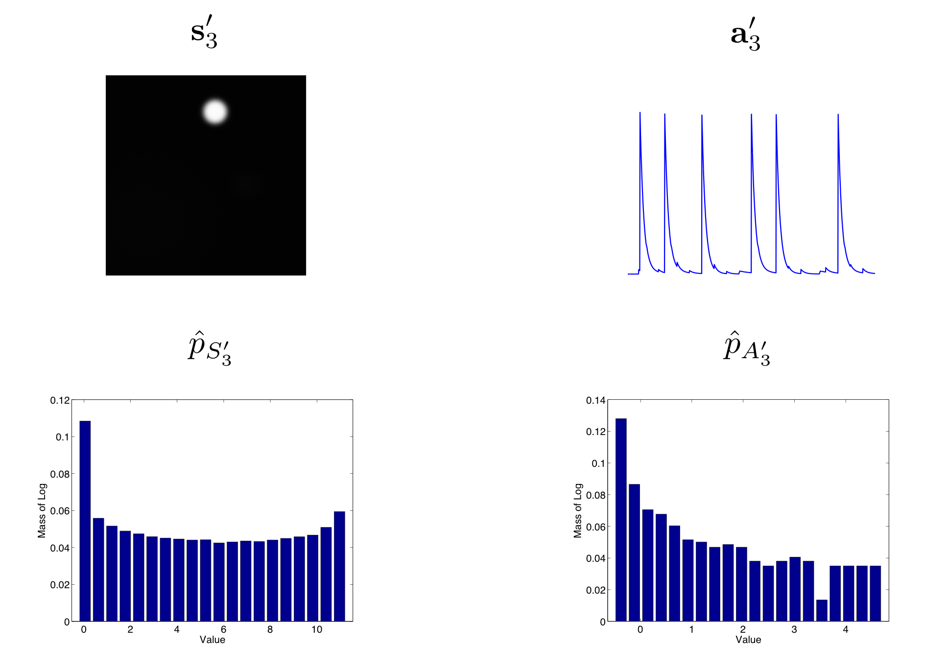
Figure: ICA Model

Here we show the estimate independent image and trace component and their corresponding empirical distributions. In order to highlight the skewness of the distribution we use the normalized log histogram $\hat{p}$ for the empirical distribution. In this case, the skewness of both the image and trace distributions is positive.

Unmixing Images and Traces¶

The ICA algorithm gives us an unmixing matrix $\hat{\mathbf{F}}$. The ICA Unmixing Dimension option allows us to control how $\hat{\mathbf{F}}$ is used to get the output of this algorithm.

This choice will cause the outputs of the algorithm to have different properties, such as their signal-to-noise ratio and mutual correlation or orthogonality.

Temporal¶

In this case, we apply the unmixing matrix to the principal traces:

\[ \hat{\mathbf{A}} = \mathbf{V}' \hat{\mathbf{F}} \]

to get a set of traces that represent the activity of each component.

We then project the zero-mean movie matrix $\mathbf{M}'$ onto these traces to get a set of images:

\[ \hat{\mathbf{S}} = \mathbf{M}' \hat{\mathbf{A}} \]

which define where each component's activity is taking place.

Finally, we compute a set of images that can be used to approximately reconstruct the traces $\hat{\mathbf{A}}$ from the movie matrix $\mathbf{M}'$ by computing the Moore-Penrose pseudoinverse of $\hat{\mathbf{S}}$:

\[ \mathbf{S}^{+} = \left( \hat{\mathbf{S}}^\top \hat{\mathbf{S}} \right)^{-1} \hat{\mathbf{S}}^\top. \]

ICA then outputs those images $\mathbf{S}^+$ and the traces $\hat{\mathbf{A}}$.

These traces should be less noisy than those obtained with Spatial, so are more powerful as input to eventDetection. However, the traces are also mutually orthogonal or uncorrelated and so may not be suitable for other analyses.

Another advantage of this option is that the zero-mean movie, the traces, and the images are consistent in the sense that the traces are approximately the product of the other two:

\[ \mathbf{S}^+ \mathbf{M}' \approx \hat{\mathbf{A}} \]

though it is not true that the movie is approximately equal to the product of the images and traces.

Spatial¶

In this case we apply the unmixing matrix to the principal images:

\[ \hat{\mathbf{S}} = \mathbf{U}' \hat{\mathbf{F}} \]

to get a set of images that represent where each component is spatially defined.

We then project the zero-mean movie matrix $\mathbf{M}'$ onto these images to get a set of traces

\[ \hat{\mathbf{A}} = \mathbf{M}'^\top \hat{\mathbf{S}} \]

to define the temporal activity associated with those images.

ICA then outputs the images $\hat{\mathbf{S}}$ and the traces $\hat{\mathbf{A}}$.

One advantage of this option is that the zero-mean movie, the traces and the images are consistent in the sense that the traces are approximately the product of the other two:

\[ \hat{\mathbf{S}}^\top \mathbf{M}' \approx \hat{\mathbf{A}} \]

and that the movie is approximately equal to the product of the images and traces:

\[ \mathbf{M}' \approx \hat{\mathbf{S}} \hat{\mathbf{A}}^\top. \]

The disadvantage of this option is that the traces will be noiser than those obtained by Temporal and may contain more confounding signals. However, the traces will not necessarily be mutually orthogonal or uncorrelated and so would be more suitable for general analyses.

Both¶

In this case we apply the unmixing matrix to both the principal images and traces

\[ \hat{\mathbf{S}} = \mathbf{U}' \hat{\mathbf{F}} \\ \hat{\mathbf{A}} = \mathbf{V}' \hat{\mathbf{F}} \]

ICA then outputs the images $\hat{\mathbf{S}}$ the traces $\hat{\mathbf{A}}$.

The main advantage of this option is that it produces the least noisy traces and images.

The main disadvantage is that, like Temporal, it always produces traces that are mutually uncorrelated. Another disadvantage is that, unlike Temporal and Spatial, there is no consistent relationship between the zero-mean movie, traces and images.

Mukamel 2009, Automated Analysis of Cellular Signals from Large-Scale Calcium Imaging Data ↩↩↩↩