CNMF-E
This tool uses 2.0 compute credits per hour.
CNMF-E is a constrained non-negative matrix factorization (CNMF) algorithm used to perform automated source extraction from microendoscopic calcium imaging movies. Specifically, it aims to retrieve the spatial location and temporal dynamics of neurons in a fluorescent 1-photon calcium imaging movie.
Inputs
| Parameter | Required? | Default | Description |
|---|---|---|---|
| Input Movie Files | True | N/A | Path to the input isxd movie files |
| Cell Diameter | True | 7 | Average cell diameter of a representative cell in pixels |
| Minimum Correlation | True | 0.8 | Minimum correlation of a pixel with its immediate neighbors when searching for new cell centers |
| Minimum Peak-to-Noise Ratio | True | 10 | Minimum peak-to-noise ratio of a pixel when searching for new cell centers. |
| Background Spatial Subsampling | True | 2 | Spatial downsampling factor to use when estimating the background activity |
| Ring Size Factor | True | 1.4 | Multiple of the average cell diameter to use for computing the radius of the ring model used for estimating the background activity |
| Gaussian Kernel Size | True | 0 | Width in pixels of the Gaussian kernel used for spatial filtering of the movie before cell initialization (automatically estimated when the value provided is smaller than 3) |
| Closing Kernel Size | True | 0 | Size in pixels of the morphological closing kernel used for removing small disconnected components and connecting small cracks within individual cell footprints (automatically estimated when the value provided is smaller than 3) |
| Merge Threshold | True | 0.7 | Temporal correlation threshold for merging cells that are spatially close |
| Processing Mode | True | parallel_patches | Processing mode to use to run CNMF-E. 'All in memory' processes the entire field of view at once. 'Sequential patches' breaks the field of view into overlapping patches and processes them one at a time using the specified number of threads where parallelization is possible. 'Parallel patches' breaks the field of view into overlapping patches and processes them in parallel using a single thread for each. |
| Number of Threads | True | 4 | Number of threads to be used for running the CNMFe algorithm |
| Patch Size | True | 80 | Side length of an individual square patch within the field of view in pixels |
| Patch Overlap | True | 20 | Amount of overlap between adjacent patches in pixels |
| Output Unit Type | True | df_over_noise | Units of the output temporal traces. 'dF' will produce temporal traces on the same scale of pixel intensity as the original movie. dF is calculated as the average fluorescence activity of all pixels in a cell, scaled so that each spatial footprint has a magnitude of 1. 'dF over noise' will produce temporal traces divided by their respective estimated noise level. This can be interpreted similarly to a z-score, with the added benefit that the noise is a more robust measure of the variance in a temporal trace compared to the standard deviation. |
Our Parameter Setting Tips page can be consulted to gain insights and tips to fine-tune CNMF-E parameters to optimize performance.
File Inputs
| Source Parameter | File Type | File Format |
|---|---|---|
| Input Movie Files | miniscope_movie, miniscope_movie | isxd, isxc |
Background
The CNMF algorithm was originally developed for two-photon data by Pnevmatikakis, 20161. The two-photon algorithm was modified with enhanced background subtraction routines to work in the one-photon setting by Zhou, 20182. The first version of CNMF-E, originally developed in MATLAB as CNMF_E, was ported to Python in the CaImAn package, described in Giovannucci, 20183. The Inscopix Data Products and Analytics team then reimplemented the constrained non-negative matrix factorization approach in C++ (Inscopix CNMF-E) for implementation into Inscopix Data Processing Software, improved for performance, and extended to offer greater processing control and transparency.
Algorithm Overview
CNMF-E is an iterative algorithm that solves a non-convex optimization problem, which consists of minimizing the difference between the input movie and the data reconstructed using the model. The process consists of making an initial estimation of the spatial location and temporal activity of cells, which we refer to as the initialization phase, and then refining this estimate over several iterations of processing. The algorithm can be broken down into distinct and reusable processing modules as depicted below.
The first two steps of Inscopix CNMF-E aim to determine how to efficiently process the movie through division of labor and efficient memory management. The following 13 steps (steps 3 through 16) encompass the core functionality of CNMF-E and are applied to the movie, or to spatially distinct portions of the movie for parallel processing. Finally, the results from parallel processing are combined and the components scaled based on user-specified parameters.
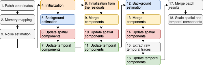
Figure: Overview of the CNMFe algorithm.
Colors highlight repeated modules.
Determine patch coordinates
Based on the chosen mode, the field of view may be broken up into spatially distinct regions referred to as patches. This first step determines the boundaries of all such patches based on the specified patch size and patch overlap.
Create memory-mapped files
The next step is to convert one or more .isxd movie files into memory-mapped files, allowing efficient memory management and processing of files otherwise too large to fit in memory at once.
Noise estimation
The power spectrum of each pixel is computed by applying a fast Fourier transform to its temporal variation, and then averaged over the high-frequency range to estimate the noise level.
Cell initialization
In the next step, each frame of the movie is first high-pass filtered with a Gaussian filter of size equal to Gaussian filter width. The correlation and peak-to-noise ratio (PNR) images are computed from the filtered movie. The correlation image is an image where a particular pixel value is equal to the average correlation over time of that pixel with the 8 neighbor pixels that surround it. The PNR image is an image where a pixel value is equal to the maximum value over time divided by the estimated noise level. A search image is constructed by multiplying the correlation and PNR images. Here's an example from a striatal recording of what these images look like:
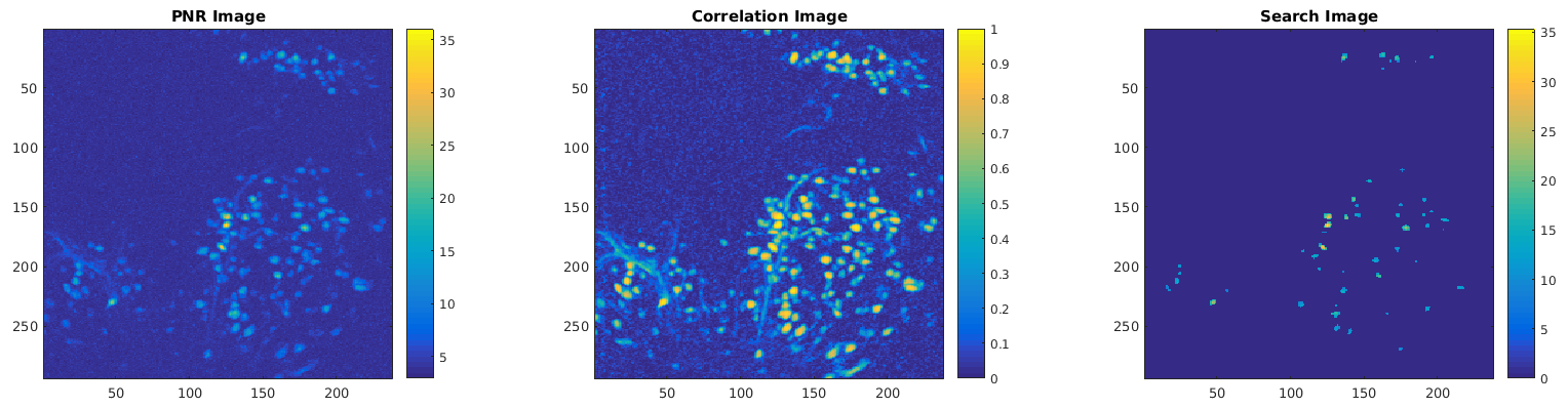
A good initialization is essential for good cell identification, and the Min pixel correlation and Min peak-to-noise ratio parameters are the primary parameters used in the initialization process. First, the correlation and PNR images are thresholded by the Min pixel correlation and Min peak-to-noise ratio parameters, and the search image is computed by multiplying the two thresholded images. In the figure above, the PNR and correlation images are shown before thresholding, the search image is shown after. The threshold parameters were Min pixel correlation=0.8 and Min peak-to-noise ratio=5.
After computing the search image, the highest valued pixel is selected as a seed pixel, and the seed pixel is considered to be a potential cell. A box around the seed pixel is constructed, roughly the size of the parameter Average cell diameter, and a basic footprint and trace extraction is performed. The cell footprint is subtracted from from the search image, and the process is repeated until no more seed pixels are found.
Background estimation
After CNMF-E obtains an initialization for the footprints and traces, it estimates the background, with the footprints and traces fixed. The background estimation uses a "ring model", in which the background at a pixel is estimated as a linear combination of activity for a ring around that pixel, with diameter equal to Ring size factor times the cell size as specified by Average cell diameter. Figure 5a from 4, reproduced here with permission, can provide some intuition about the background model:
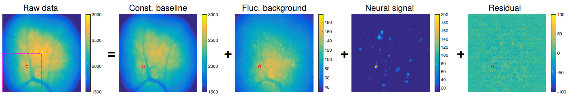
This figure shows the raw data (left) being composed of a static background image ("const. baseline"), a time-varying background computed with the ring model ("Fluc. background"), the actual neural signal comprised of the footprints and traces, and then the residual, which is whatever is left.
Update the spatial footprints
The estimated background is subtracted from the movie, and the footprints are re-fit, using a constrained non-negative matrix factorization (CNMF) approach, with each footprint that resulted from the initialization step serving as the initial guess to the CNMF optimization. After a footprint is refined in this way, it is post-processed. The post-processing steps include smoothing with a median filter, morphological closing, and thresholding, followed by retaining only the largest connected component.
Update the temporal traces
In this step, the spatial footprints and background are fixed, and the traces for each cell are optimized in parallel. Each trace is denoised using a deconvolution algorithm as described in 5. The deconvolution is accomplished by modeling the generation of calcium traces from spikes using a simple exponential model. The following figure illustrates example traces with deconvolved spike events:
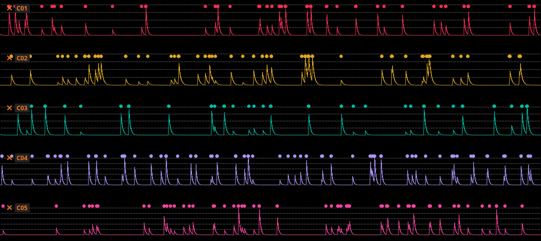
The algorithm implementation of 5 does not produce discrete unit-valued spikes as output; the spikes have an amplitude that ranges from zero to one. "True" spikes tend to have values that are closer to one than "noise" spikes. Spikes can be thresholded to produce events that appear to correspond better to increments in the calcium trace.
Cell merging
A merging algorithm is executed after each iteration of spatial/temporal fitting. The algorithm looks for cells that are spatially close and whose traces have high temporal correlations. Cells with a temporal correlation greater than the parameter Merging threshold are automatically merged throughout the process.
Extract raw temporal traces
The residual of each temporal trace is computed and added back to the denoised trace to obtain a raw version of the trace.
Merge results from all patches
In this step, the results of all independent patches are combined into a single set of spatial footprints and temporal traces. Duplicate cells that can arise when using a patch overlap greater than zero are removed by keeping cells only if their closest patch center matches the patch in which they were identified.
Scale spatial footprints and temporal traces
The spatial footprints are vectorized and normalized to have unit length. The corresponding temporal traces are then scaled based on the specified output units.
Cell filtering
The first line of defense against false positive cells is through setting the Min pixel correlation and Min peak-to-noise ratio parameters, which affect the initialization of footprints and traces. After initialization, cells can be filtered using the Spatial Bandpass Filter tool.
Troubleshooting
Our Common Issues page can be consulted for additional troubleshooting tips.
FAQ
What is the formula for dF/noise output units?
The formula to calculate df/noise is as follows:
Let K represent the number of cells, T represent the number of frames in the movie, and d represent the number of pixels in each frame. Let A represent the raw spatial footprints with dimensions d x K. Let C represent the raw temporal traces K x T.
For both df and df/noise, the spatial footprints are scaled in the following way:
nA = sqrt(sum(square(A))).transpose()
A = A * diag(1.0 / nA)
Here nA is a column vector of size K, where each entry of nA represents the magnitude of the spatial footprint of a neuron in units of pixel intensity (remember that spatial footprints are extracted from the original raw movie). The spatial footprints A are normalized to be unit vectors by dividing by nA.
For df/noise, the temporal traces are scaled in the following way:
for k in range(K):
  sn = get_noise_fft(
    trace=C[k, :],
    noise_range=[0.25, 0.5],
    noise_method="mean"
  )
  C[k, :] /= sn
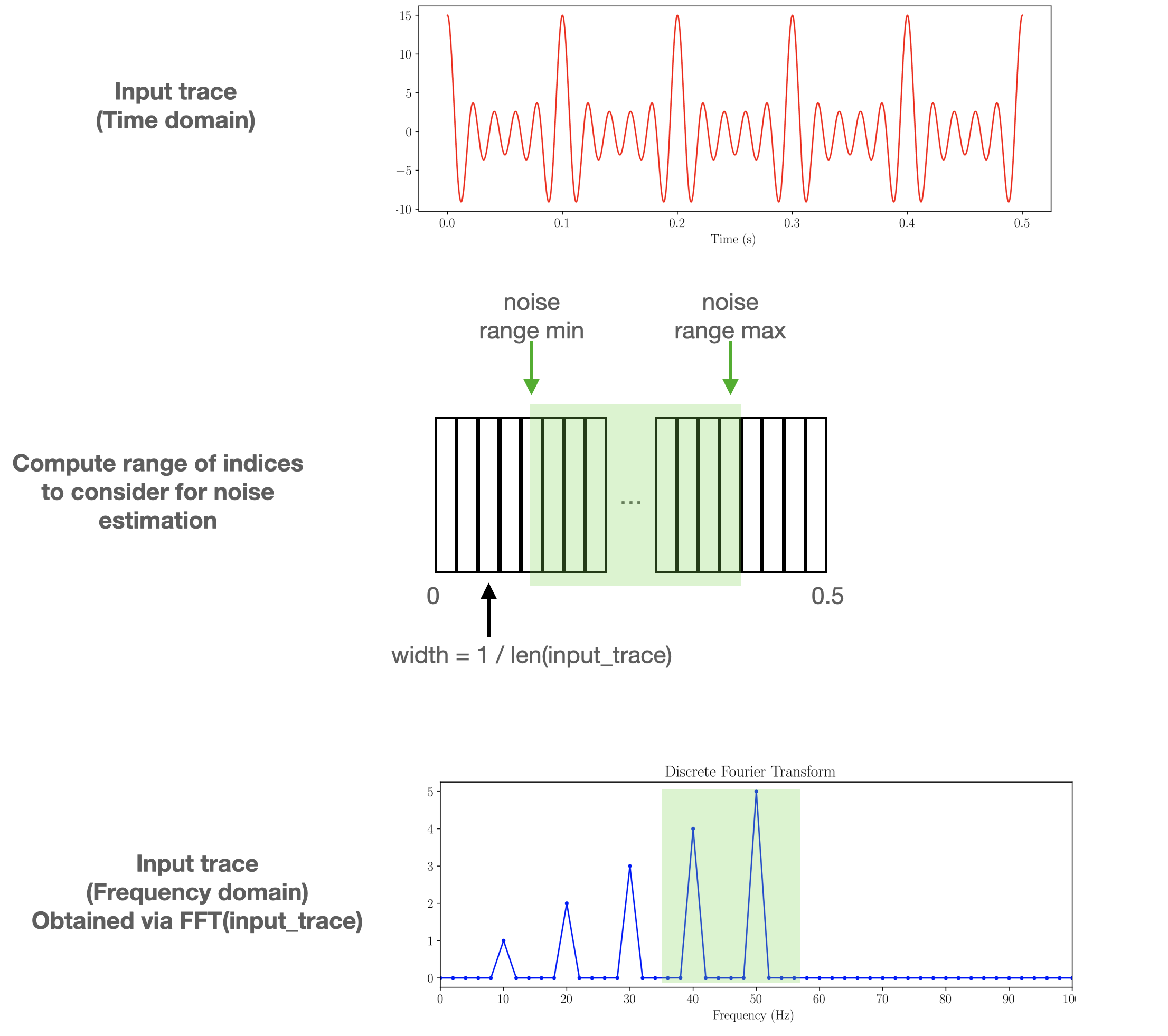
For each temporal trace, the noise is computed using a fast fourier transform, and the trace is scaled by this noise estimate.
get_noise_fft computes noise by calculating the power spectral density of the trace using a FFT, over a desired noise range (hardcoded, not configurable by the user). This PSD is then averaged using mean. Here’s a diagram to demonstrates how noise is computed this way:
-
Pnevmatikakis 2016, Simultaneous Denoising, Deconvolution, and Demixing of Calcium Imaging Data ↩
-
Zhou 2018, Efficient and accurate extraction of in vivo calcium signals from microendoscopic video data ↩
-
Giovannucci 2018, CaImAn an open source tool for scalable calcium imaging data analysis ↩
-
Efficient and accurate extraction of in vivo calcium signals from microendoscopic video data ↩
-
Friedrich 2017,Fast online deconvolution of calcium imaging data ↩↩