Estimate Vessel Diameter¶

This tool uses 0.5 compute credits per hour.

Use this tool to measure the diameter of individual blood vessels over time from a movie. The output of this tool is a vessel set containing the selected regions of interest, defined by lines drawn across vessels and perpendicular to the blood flow, and traces representing the diameter of each vessel over time. A projection image of the movie is also stored in the vessel set.

Inputs¶

Parameter	Required?	Default	Description
Input Movies Files	True	N/A	The input isxd, blood flow, movie files.
Line ROIs	True	N/A	Draw lines across vessels of interest perpendicular to the direction of blood flow, 2-3x longer than the diameter of the vessel. Overlap with neighboring vessel or other bright features must be avoided.
Time Window	True	2	The duration in seconds of the time window to use for every measurement.
Time Increment	True	1	The time shift in seconds between consecutive measurements. When the time increment is smaller than the time window, consecutive windows will overlap. The time increment must be less than or equal to the time window.
Output Units	True	pixels	Output units for vessel diameter estimation.
Estimation Method	True	Non-Parametric FWHM	The type of method to use for vessel diameter estimation. Both methods estimate diameter from a line profile extracted from the input movie using the input contours. Parametric FWHM fits the line profile to a Lorentzian curve. Non-Parametric FWHM measures the distance between the midpoints of the line profile peak.
Height Estimate Rule	True	independent	Used in Non-Parametric FWHM estimation method. Describes the method to use for determing the midpoint height on each side of the line profile peak. If 'Global', take the halfway point between the max and the global min. If 'Local', take the largest of the two halfway points between min/max. If 'Independent', the height estimate will be independent on both sides of the peak.
Auto Accept/Reject	True	True	Flag indicating whether the vessels should be auto accepted/rejected. Rejected vessels are identified as those with derivatives greater than a particular fraction of the mean.
Rejection Threshold Fraction	True	0.2	Parameter for auto accept/reject functionality. The max fraction of the mean diameter allowed for a derivative in a particular vessel diameter trace.
Rejection Threshold Count	True	5	Parameter for auto accept/reject functionality. The number of threshold crossings allowed in a particular vessel diameter trace.

File Inputs¶

Source Parameter	File Type	File Format
Input Movies Files	miniscope_movie	isxd

Note about multiple file inputs

This tool supports multiple .isxd files in the Input Movie Files parameter. If multiple files are provided, the tool analyzes the multiple files as a single movie, and outputs one vessel set for each input movie.

Description¶

This sections provides an overview of how the algorithm estimates vessel diameter from an input movie. The user is required to supply the algorithm with regions of interest called “lines” across vessels they would like to measure. The following image shows an example of a good line that can be used as an input to the algorithm.

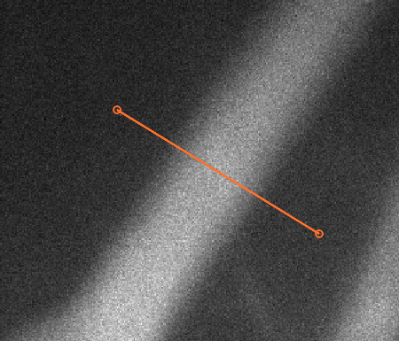
In general, a good line has the following properties:

The line is oriented along the axis of the vessel and is perpendicular to the axis of blood flow
Symmetric relative to the center of the vessel diameter
Approximately 2-3x wider than the vessel diameter
Avoiding intercepting other vessels where possible

Each user line is provided as input to the algorithm. For each user line, the following steps are applied to estimate diameter from the input.

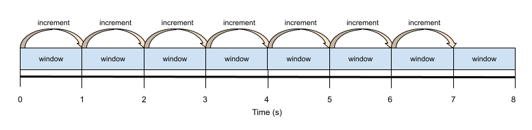
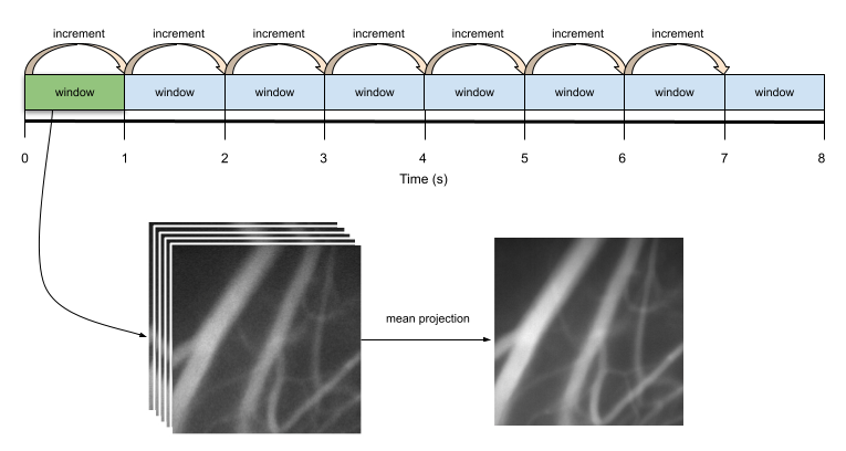
Step 1: Divide movie into windows¶

For a particular vessel, the algorithm collects multiple measurements of diameter over time by applying a sliding window on the input movie. The sliding window is parameterized by the time window and time increment parameters described in the Inputs section. The following image demonstrates an example sliding window where the time window equals the time increment. In this case, there is no gap in time between consecutive windows.

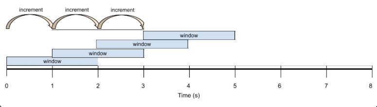
*Example windowing where time window = time increment.*

The next image demonstrates an example sliding window where the time window is greater than the time increment. In this case, there is overlap in time between consecutive windows.

Step 2: Compute mean projection image¶

To obtain a single measurement of diameter for one particular vessel, a time window is selected. All the frames in the selected time window are used to generate a mean projection image. This image represents the averages pixel values of the movie over the selected time window. The following image demonstrates this process.

*Example window highlighted in green is selected for analysis and converted into a mean projection image.*

The next steps of the algorithm will depend on the type of estimation method that’s selected as input in the algorithm.

Parametric FWHM¶

This method uses a parametric approach to estimate diameter from a line profile, based on the procedure described in Ghosh 2011¹. The steps of this approach are summarized below.

Step 3: Fit the model¶

Given a line profile, a non-linear least squares approach is used to fit a Lorentz distribution to the profile. According to Ghosh 2011¹, a Lorentzian fit was chosen because it provided superior approximation of line profiles in comparison to Gaussians based on empirical results.

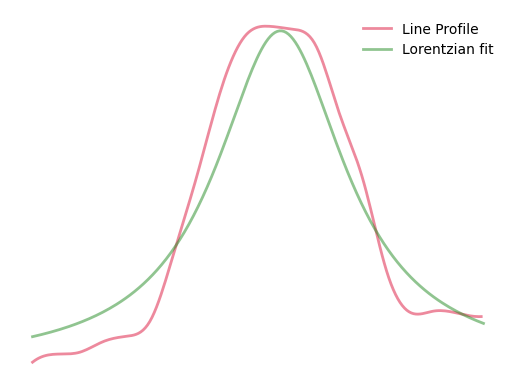
*Example line profile fit to a Lorentzian distribution.*

Step 4: Calculate diameter¶

The vessel diameter is estimated by taking the full width at half maximum (FWHM) of the Lorentzian fit curve.

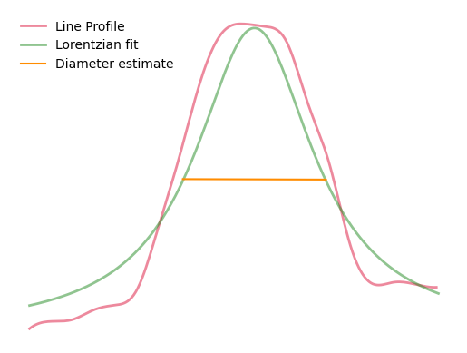
*Example diameter estimate derived from the FWHM of a Lorentzian fit to a line profile.*

Non-Parametric FWHM¶

This method uses a non-parametric approach to estimate diameter by measuring the distance between the midpoints of the line profile peak, which is described in the following steps.

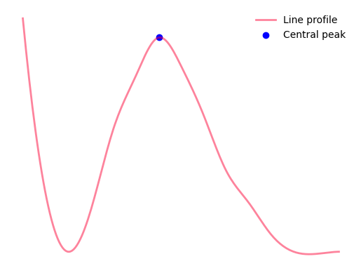
Step 3: Find central peak¶

The central peak of the vessel profile is located, demonstrated in the following image.

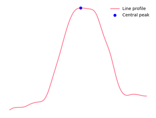
*Example central peak on a line profile, which correspond to the global max of the line profile.*

The peak must not be at either extreme of the line profile, i.e., must be somewhere in the middle of the line profile, demonstrated in the next image. This avoids the possibility that rising tails confound the diameter measurement.

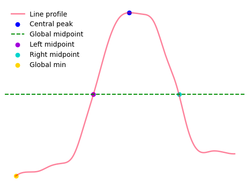
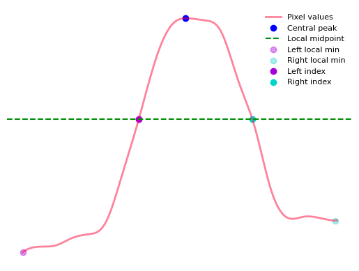
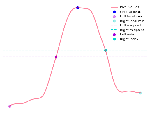
Example central peak on a line profile with a max on an extreme end. In this case, the max at the extreme end of the line profile is ignored, and the selected peak is the one near the center of the line profile.

Step 4: Find peak midpoints¶

The midpoint between the peak and minima on either side of the peak is computed. This is used as a threshold for where the diameter measurement should be taken from. For each side of the peak, the midpoint can be computed one of the following ways, depending on which height estimate rule was specified by the user in the algorithm parameters. For each midpoint, linearly interpolate the index where that height occurs. The following sub-sections describe how midpoints are computed for each height estimate rule.

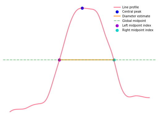
Global: Take the halfway point between the central peak and the global min. The following image shows an example of midpoints derived from a line profile using this method.

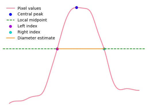
*Example midpoints estimated using the global rule.*

Local: Find the local minima on both sides of the peak and compute a halfway point between the central peak and the local minima for each side. Take the largest of these two halfway points and use this as the local midpoint. The following image shows an example of midpoints derived from a line profile using this method.

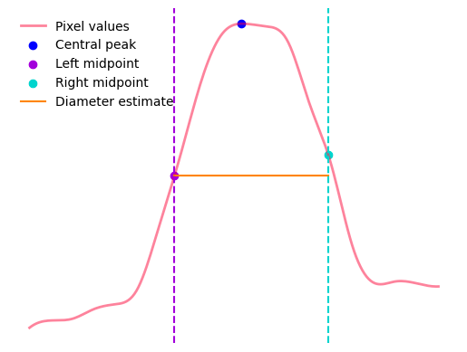
*Example midpoints estimated using the local rule.*

Independent: Find the local minima on both sides of the peak and compute a halfway point between the central peak and the local minima for each side. The height estimate will be independent on both sides of the peak according the halfway point computed for each corresponding side. The following shows an example of midpoints derived from a line profile using this method.

*Example midpoints estimated using the independent rule.*

Step 5: Calculate diameter¶

Calculate diameter as the distance between the left and right side peak midpoints. The following three images show examples of diameter estimates derived using different height estimate rules.

*Example diameter estimate from global midpoints.*

*Example diameter estimate from local midpoints.*

*Example diameter estimate from independent midpoints.*

Vessel Auto Accept/Reject Filtering¶

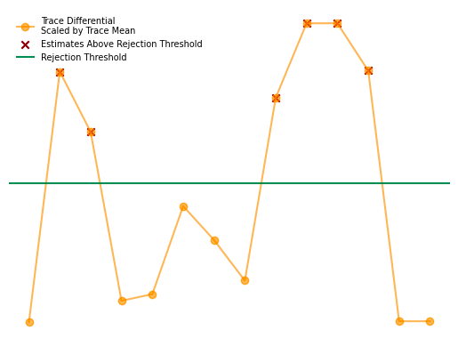
This algorithm provides an optional step to automatically accept/reject vessels, which uses the following criteria for filtering. Given a time-series trace of diameter estimates for a particular vessel, a differential of the trace is computed and then divided by the trace mean. The number of elements in this scaled differential trace which exceed the rejection threshold fraction (from the Inputs) is counted. If number of elements is greater than or equal to the rejection threshold count (from the Inputs), then the corresponding vessel is assigned a rejected status, otherwise, the vessel is assigned an accepted status.

The following image demonstrates a vessel that would be accepted by the filtering method because no elements in the scaled differential trace exceed the rejection threshold fraction.

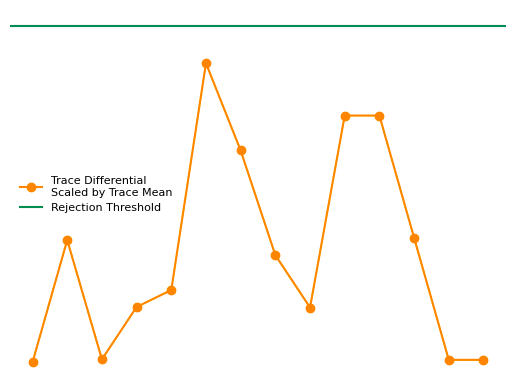
*Example of a vessel that would be accepted, since no elements in the scaled differential trace exceed the rejection threshold.*

In contrast, the next image demonstrates a vessel that would be rejected by the filtering method because there are elements in the scaled differential trace which exceed the rejection threshold fraction. The algorithm can be tuned to be more permissive by increasing the rejection threshold count, and more strict by decreasing the rejection threshold count.

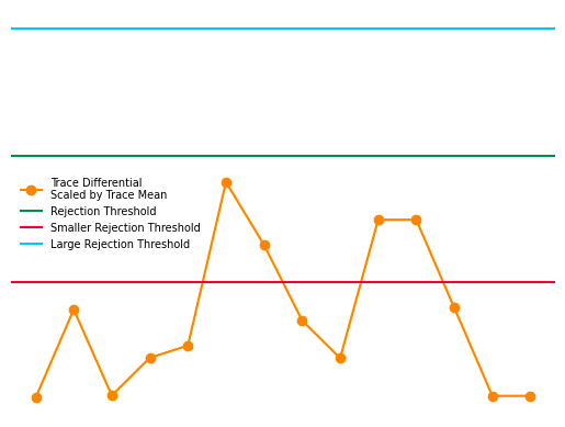
Example of a vessel that would be rejected if the rejection threshold count was less than or equal to six, since there are six elements in the scaled differential trace which exceed the rejection threshold.

Similarly, the filtering step can be tuned to be more permissive by increasing the rejection threshold fraction, and vice versa to make the step more strict. The following image demonstrates this effect.

*Example of a vessel that would be rejected or accepted depending on varying rejection threshold fractions.*

Outputs¶

The output of this tool is a vessel set object, which stores the estimated vessel diameter traces based on the input line ROIs. If multiple input files are provided, the tool outputs one vessel set file for each input movie. Two previews are generated for each vessel set file.

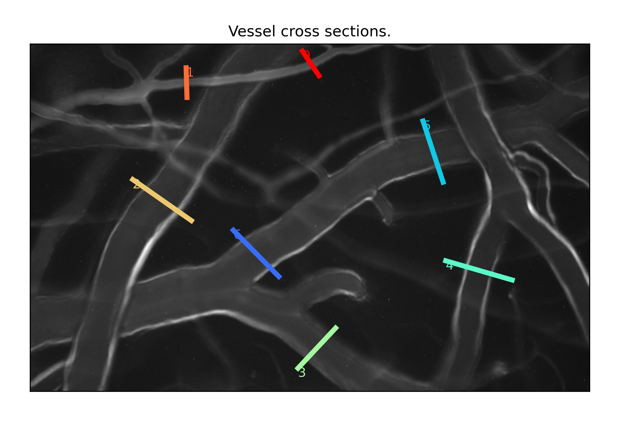
The first preview shows the line ROIs used as input to generate the vessel set. The coordinates of these line ROIs are stored in the vessel set file and can be viewed when opening the file in IDPS.

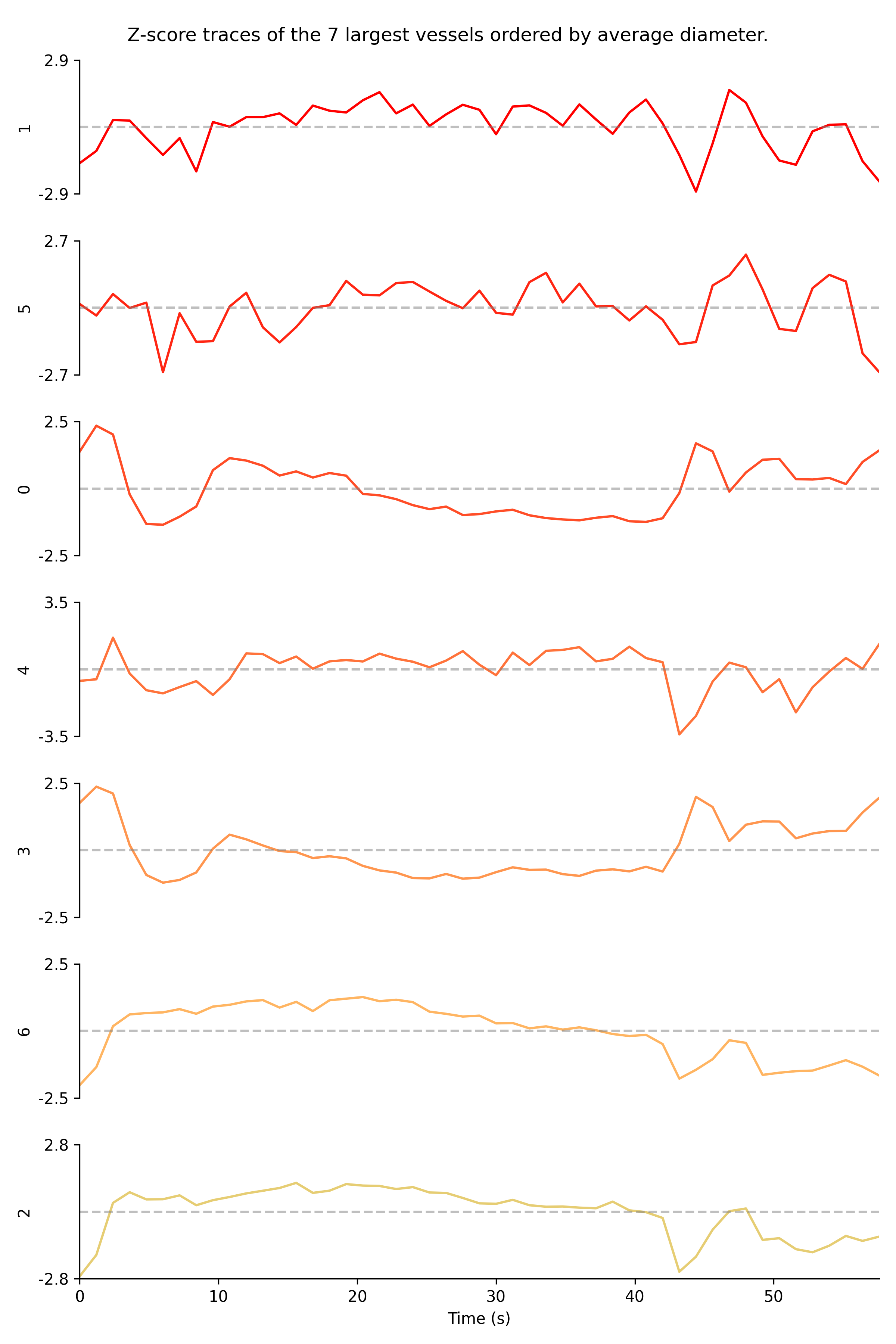
*Example preview of annotated vessel cross-sections where diameters are measured.*

The second preview shows the traces estimated by the algorithm. This preview shows a subset of the largest vessels ordered by average diameter. The traces are Z-scored to outline the changes in diameter over time.

*Example preview of Z-scored traces of diameter measurements.*

Ghosh KK, Burns LD, Cocker ED, Nimmerjahn A, Ziv Y, Gamal AE, Schnitzer MJ. Miniaturized integration of a fluorescence microscope. Nat Methods. 2011 Sep 11;8(10):871-8. ↩↩