Combine and Compare Neural Activity Across Epochs
This tool uses 1.0 compute credits per hour.
Overview
This tool combines trace, events, and correlation metrics during different epochs from the Compare Neural Activity Across Epochs tool from multiple recordings and statistically compares them using ANOVA. If only one group is provided, the tool will calculate a 1-way ANOVA, as well as pair-wise comparisons between the epochs. If two groups are provided, the tool will calculate a 1-way ANOVA for each group, as well as a 2-way mixed-design ANOVA to compare the two groups. The tool will also perform pair-wise comparisons between the groups for each epoch, calculating the effect size and significance.
The tool will perform separate comparisons for the average trace activity, event rate, average positive correlation, and average negative correlation. The event rate and correlation files are optional, and the tool will only perform the comparisons for the files that are provided.
To perform the statistical test, the user can choose:
- Which multiple-comparison correction method to use (Bonferroni, Sidak, Holm, Benjamini-Hochberg, or Benjamini-Yekutieli, or none).
- Which effect size to calculate (Cohen's d, Hedges' g, r, eta-squared, odds ratio, area under the curve, or Common Language Effect Size).
Parameters
| Parameter | Required? | Default | Description |
|---|---|---|---|
| Group 1 Trace Files | True | N/A | Group 1 Trace Files |
| Group 2 Trace Files | False | N/A | Group 2 Trace Files |
| Group 1 Eventrate Files | False | N/A | Group 1 Eventrate Files |
| Group 2 Eventrate Files | False | N/A | Group 2 Eventrate Files |
| Group 1 Correlation Files | False | N/A | Group 1 Correlation Files |
| Group 2 Correlation Files | False | N/A | Group 2 Correlation Files |
| Name of Epochs | True | Epoch 1, Epoch 2, Epoch 3 | List of names of epochs |
| Name of the first group | True | N/A | Name of the first group |
| Name of the second group | False | N/A | Name of the second group |
| Epoch Color Palette | True | tab:grey, tab:blue, tab:cyan | List of matplotlib compatible colors to represent each epoch |
| Color of the first group | True | tab:red | Color of the first group |
| Color of the second group | True | tab:orange | Color of the second group |
| Multiple Comparison Correction Method | True | bonf | Method to correct for multiple comparisons |
| Effect Size Method | True | cohen | Method to calculate effect size |
Input Files
The inputs to this tool are a list of epoch activity metrics files that are generated from the Compare Neural Activity Across Epochs tool.
Input Requirements
-
If a group recieves data, that group must contain at least two recordings, otherwise the tool will terminate.
-
All input files must be generated using the same number of epochs, using the same epoch names. However, the length of the epochs can vary between recordings.
-
If your epoch name is only a number, extra characters such as
+, or a trailing.0may be trunacted from the label due to how the number is processed by thepandaspackage before being converted to a string.
| Source Parameter | File Type | File Format |
|---|---|---|
| Group 1 Trace Files | epoch_activity_data | csv |
| Group 2 Trace Files | epoch_activity_data | csv |
| Group 1 Eventrate Files | epoch_activity_data | csv |
| Group 2 Eventrate Files | epoch_activity_data | csv |
| Group 1 Correlation Files | epoch_activity_data | npy |
| Group 2 Correlation Files | epoch_activity_data | npy |
Algorithm Description
The tool is summarized using a flowchart below.
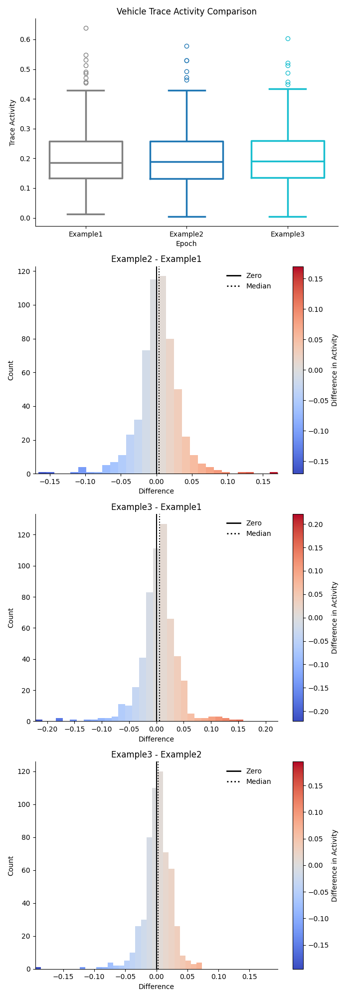
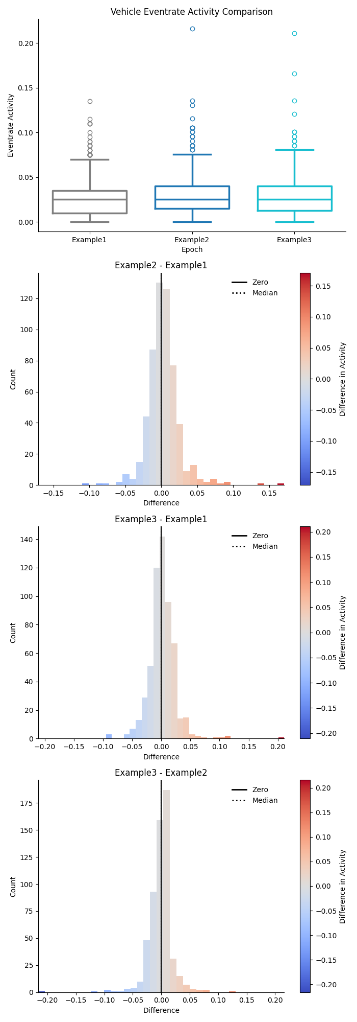
The tool begins by combining the data from each group. Then the two groups are compared to determine if there is statistically significant difference between average trace activity levels, the eventrate, the average positive correlation, or the average negative correlation.
Combination
The combination step is performed independently for each input group. The combination step concatenates the data from each recording end to end, retaining all original columns, adds a column to indicate the source file, and a column indicating the datatype of the cell.
1-way ANOVA
The 1-way ANOVA is performed for each group and each metric (trace, event rate, positive correlation, negative correlation) to determine if there is a significant difference between the epochs. The ANOVA is performed using the pingouin.anova function from the pingouin package.
Mixed-Design ANOVA
The mixed-design ANOVA is performed when two groups are provided. The mixed-design ANOVA is performed using the pingouin.mixed_anova function from the pingouin package. The mixed-design ANOVA is used to determine if there is a significant difference between the groups, epochs, and the interaction between the two.
Pairwise Comparisons
Before any comparisons are made, the data is checked for normality using the Shapiro-Wilk test. If the data is not normally distributed, the Wilcoxon signed-rank test is used instead of the t-test.
The pairwise comparisons are made using the pingouin.pairwise_ttests function from the pingouin package. The effect size and multiple comparison correction used are determined by the user.
Effect Size Calculation Options
| Method | Description |
|---|---|
| Cohen's d | A measure of effect size that expresses the difference between two means in standard deviation units. |
| Hedges' g | Similar to Cohen's d, but includes a correction for small sample sizes, providing a more accurate estimate of effect size. |
| r eta-squared (η²) | A measure of the proportion of variance in a dependent variable that is associated with one or more independent variables. |
| Odds ratio | A measure of association between two binary variables, representing the odds of an event occurring in one group versus another. |
| Area under the curve (AUC) | Typically refers to the AUC of a receiver operating characteristic (ROC) curve, used to evaluate the performance of a binary classifier by measuring its ability to distinguish between classes. |
| Common Language Effect Size | A probability-based effect size that expresses the likelihood that a randomly chosen score from one group will be higher than a randomly chosen score from another group. |
Multiple Comparison Correction Options
| Method | Description |
|---|---|
| Bonferroni | A correction method that adjusts the p-value threshold by dividing it by the number of comparisons, controlling for Type I errors in multiple testing. |
| Sidak | A correction method similar to Bonferroni but less conservative, adjusting p-values assuming the tests are independent. |
| Holm | A step-down method that sequentially adjusts p-values to control the family-wise error rate, providing more power than Bonferroni. |
| Benjamini-Hochberg | A method that controls the false discovery rate (FDR) by ranking p-values and applying a less stringent correction, increasing power in large datasets. |
| Benjamini-Yekutieli | An extension of the Benjamini-Hochberg procedure that controls the FDR under dependency assumptions among tests. |
| None | No correction is applied to the p-values, which increases the likelihood of Type I errors in multiple testing. |
Outputs
Combination Outputs
Combination Data
A csv file containing the combined trace and event rate data from all recordings in each group. Here is an example outputs:
| Epoch | Cell | Trace Activity | Trace file | Eventrate Activity | Eventrate file |
|---|---|---|---|---|---|
| Example1 | 0 | 0.0738 | Traces1.csv | 0.0000 | Eventrate1.csv |
| Example1 | 1 | 0.0650 | Traces1.csv | 0.0050 | Eventrate1.csv |
| Example1 | 2 | 0.1505 | Traces1.csv | 0.0550 | Eventrate1.csv |
| Example1 | 3 | 0.0641 | Traces1.csv | 0.0150 | Eventrate1.csv |
| Example1 | 4 | 0.0893 | Traces1.csv | 0.0050 | Eventrate1.csv |
Combination Previews
The combination figures will show a separate preview for both trace activity and event rate in each group as a box plot in the top row, and the pairwise difference in activity between each combination of epochs in the subsequent rows.
Correlation Combination Data
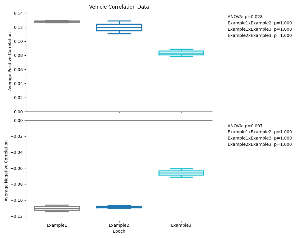
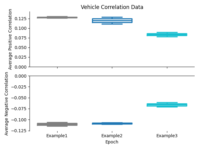
The correlation data is combined separately because we are comparing the average positive and negative correlation from each recording rather than a per cell measurement. Below is an example output:
| file | Epoch | Average Positive Correlation | Average Negative Correlation |
|---|---|---|---|
| correlation_file_1.npy | Example1 | 0.130 | -0.106 |
| correlation_file_1.npy | Example2 | 0.129 | -0.110 |
| correlation_file_1.npy | Example3 | 0.078 | -0.061 |
| correlation_file_2.npy | Example1 | 0.126 | -0.114 |
| correlation_file_2.npy | Example2 | 0.111 | -0.107 |
| correlation_file_2.npy | Example3 | 0.089 | -0.071 |
Correlation Combination Previews
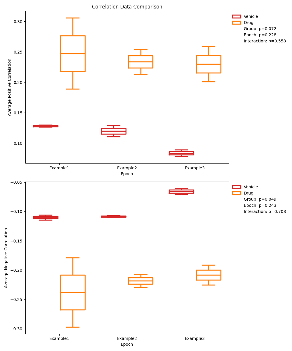
The combination figures will show a preview of the average positive correlation and average negative correlation in each group as a box plot.
ANOVA Comparison Ouputs
The ANOVA comparison outputs will show the results of both the 1-way ANOVA and the 2-way mixed-design ANOVA for all metrics. Here is an example output:
| Comparison | Source | SS | DF1 | DF2 | MS | F | p-unc | np2 | eps |
|---|---|---|---|---|---|---|---|---|---|
| Trace | Group | 0.0382 | 1 | 2 | 0.0382 | 1.9128 | 0.3008 | 0.4889 | |
| Trace | Epoch | 0.0003 | 2 | 4 | 0.0001 | 0.5938 | 0.5946 | 0.2289 | 0.5585 |
| Trace | Interaction | 0.0002 | 2 | 4 | 0.0001 | 0.5002 | 0.6399 | 0.2001 | |
| Event | Group | 0.0004 | 1 | 2 | 0.0004 | 0.2006 | 0.6981 | 0.0912 | |
| Event | Epoch | 0.0010 | 2 | 4 | 0.0005 | 0.8253 | 0.5011 | 0.2921 | 0.5049 |
| Event | Interaction | 0.0013 | 2 | 4 | 0.0006 | 1.0903 | 0.4189 | 0.3528 | |
| Positive Correlation | Group | 0.0481 | 1 | 2 | 0.0481 | 12.3190 | 0.0725 | 0.8603 | |
| Positive Correlation | Epoch | 0.0020 | 2 | 4 | 0.0010 | 2.1840 | 0.2285 | 0.5220 | 0.8948 |
| Positive Correlation | Interaction | 0.0006 | 2 | 4 | 0.0003 | 0.6762 | 0.5585 | 0.2527 | |
| Negative Correlation | Group | 0.0481 | 1 | 2 | 0.0481 | 18.8521 | 0.0492 | 0.9041 | |
| Negative Correlation | Epoch | 0.0029 | 2 | 4 | 0.0015 | 2.0584 | 0.2429 | 0.5072 | 0.6889 |
| Negative Correlation | Interaction | 0.0005 | 2 | 4 | 0.0003 | 0.3761 | 0.7085 | 0.1583 |
Here is a description of the columns:
| Column Name | Description |
|---|---|
| Comparison | The metric being compared (Trace, Event, Positive Correlation, Negative Correlation) |
| Source | The source of the variance (Group, Epoch, Interaction) |
| SS | The sum of squares |
| DF1 | The degrees of freedom for each source of variation. |
| DF2 | The degrees of freedom associated with the residual error (i.e., the variance that is not explained by the model) |
| MS | The mean square (SS / DF1) |
| F | The F-statistic |
| p-unc | The uncorrected p-value |
| np2 | The partial eta-squared effect size |
| eps | The epsilon value, which is a measure of sphericity |
Mixed-Design ANOVA Previews
The mixed-design ANOVA figures will show a preview of the data in each group and epoch, colored by group. It will also display the p-values of the Group, Epoch, and Interaction effects.
There will be a separate figure for each metric (trace, event rate, correlation).


Pairwise Comparison Outputs
The pairwise comparison outputs will show the results of both the single group pairwise comparisons and the two group pairwise comparisons for all metrics. Here is an example output:
| Comparison | Contrast | Epoch | A | B | Paired | Parametric | T | dof | alternative | p-unc | p-corr | p-adjust | BF10 | CLES |
|---|---|---|---|---|---|---|---|---|---|---|---|---|---|---|
| Trace | Epoch | - | Example1 | Example2 | True | True | 0.9071 | 3.0 | two-sided | 0.4312 | 1.0 | holm | 0.580 | 0.5000 |
| Trace | Epoch | - | Example1 | Example3 | True | True | 0.8047 | 3.0 | two-sided | 0.4799 | 1.0 | holm | 0.547 | 0.5000 |
| Trace | Epoch | - | Example2 | Example3 | True | True | -0.3591 | 3.0 | two-sided | 0.7433 | 1.0 | holm | 0.451 | 0.4375 |
| Trace | Group | - | Drug | Vehicle | False | True | 1.3830 | 2.0 | two-sided | 0.3008 | 0.912 | 1.0000 | ||
| Trace | Epoch * Group | Example1 | Drug | Vehicle | False | True | 1.2697 | 2.0 | two-sided | 0.3319 | 0.8114 | holm | 0.873 | 1.0000 |
| Trace | Epoch * Group | Example2 | Drug | Vehicle | False | True | 1.4023 | 2.0 | two-sided | 0.2959 | 0.8114 | holm | 0.919 | 1.0000 |
| Trace | Epoch * Group | Example3 | Drug | Vehicle | False | True | 1.5084 | 2.0 | two-sided | 0.2705 | 0.8114 | holm | 0.958 | 1.0000 |
| Event | Epoch | - | Example1 | Example2 | True | True | 0.5609 | 3.0 | two-sided | 0.6140 | 1.0 | holm | 0.485 | 0.4375 |
Here is a description of the columns:
| Column Name | Description |
|---|---|
| Comparison | The metric being compared (Trace, Event, Positive Correlation, Negative Correlation) |
| Contrast | The type of contrast being made |
| Epoch | The epoch being compared |
| A | The first group being compared |
| B | The second group being compared |
| Paired | Whether the comparison is paired |
| Parametric | Whether the comparison is parametric |
| T | The t-statistic |
| dof | The degrees of freedom |
| alternative | The alternative hypothesis |
| p-unc | The uncorrected p-value |
| p-corr | The corrected p-value |
| p-adjust | The multiple comparison correction method |
| BF10 | The Bayes Factor |
| Effect Size | The effect size chosen to be calculated |
Pairwise Comparison Previews
The pairwise comparison figures show the same data as the ANOVA figures, but with the pairwise comparisons p-values displayed on the plot instead of the ANOVA results. The p-values displayed are the pairwise comparison of each group at each epoch.
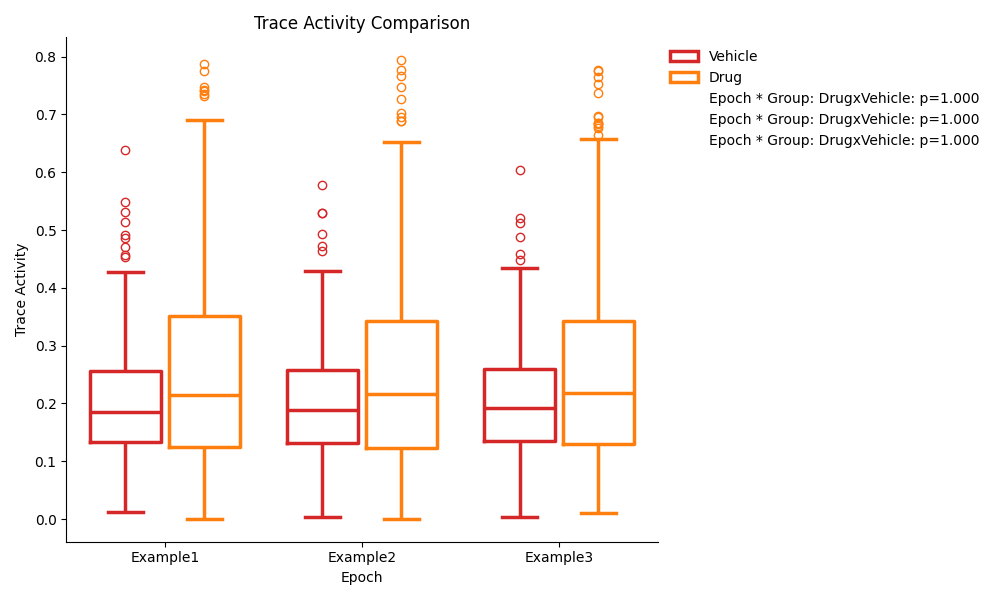
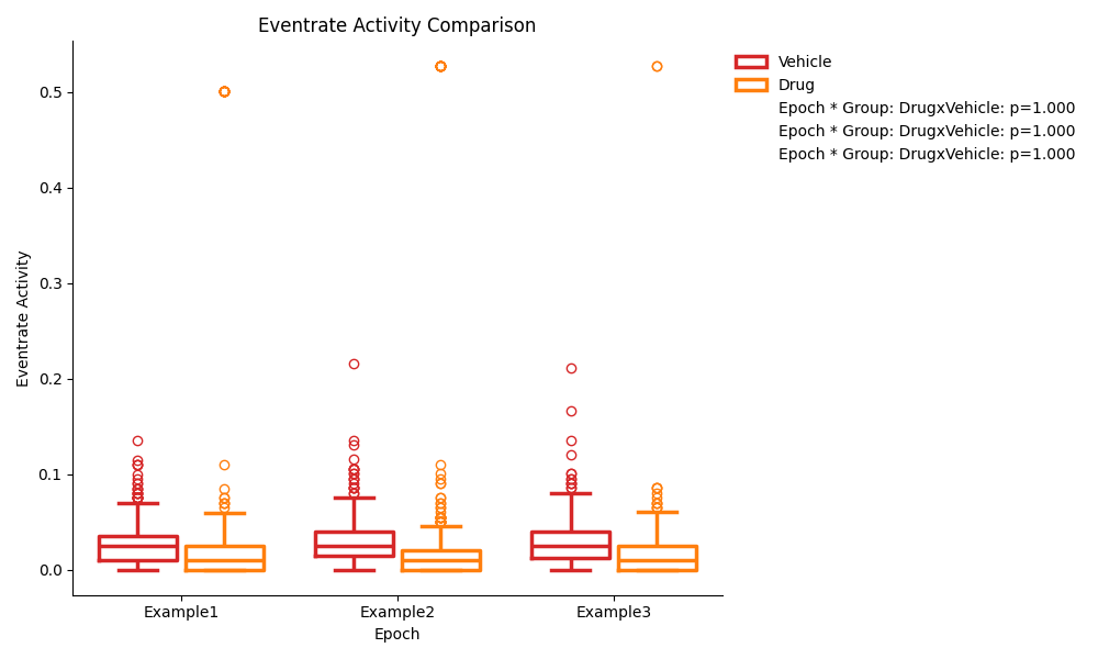
Single Group Previews
The previews for the single group comparisons will be attached to both the ANOVA and pairwise comparison outputs, because it displayed both the ANOVA results and the pairwise comparison results.